Station S3 analysis
An analysis of the environmental drivers of spring bloom timing at Station S3. This notebook works only for variables stored in pickle files created by the notebook makePickles201905.ipynb, which can be found at /ocean/aisabell/MEOPAR/Analysis-Aline/notebooks/Bloom_Timing/stationS3/makePickles201905.ipynb
To recreate this notebook, first create the pickle files, then follow the instructions in the second code cell.
[1]:
import numpy as np
import matplotlib.pyplot as plt
import matplotlib.dates as mdates
import matplotlib as mpl
import netCDF4 as nc
import datetime as dt
from salishsea_tools import evaltools as et, places, viz_tools, visualisations, bloomdrivers
import xarray as xr
import pandas as pd
import pickle
import os
import seaborn as sns
import cmocean
import pylab


%matplotlib inline
To recreate this notebook at a different location
follow these instructions:
[2]:
# The path to the directory where the pickle files are stored:
savedir='/ocean/aisabell/MEOPAR/extracted_files'
# Change 'S3' to the location of interest
loc='S3'
# What is the start year and end year+1 of the time range of interest?
startyear=2007
endyear=2021 # does NOT include this value

# Note: x and y limits on the location map may need to be changed
[3]:
modver='201905'
# lat and lon information for place:
lon,lat=places.PLACES[loc]['lon lat']
# get place information on SalishSeaCast grid:
ij,ii=places.PLACES[loc]['NEMO grid ji']
jw,iw=places.PLACES[loc]['GEM2.5 grid ji']
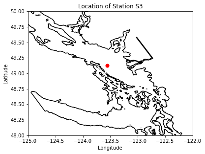
fig, ax = plt.subplots(1,1,figsize = (6,6))
with xr.open_dataset('/data/vdo/MEOPAR/NEMO-forcing/grid/mesh_mask201702.nc') as mesh:
ax.contour(mesh.nav_lon,mesh.nav_lat,mesh.tmask.isel(t=0,z=0),[0.1,],colors='k')
tmask=np.array(mesh.tmask)
gdept_1d=np.array(mesh.gdept_1d)
e3t_0=np.array(mesh.e3t_0)
ax.plot(lon, lat, '.', markersize=14, color='red')
ax.set_ylim(48,50)
ax.set_xlim(-125,-122)
ax.set_title('Location of Station %s'%loc)
ax.set_xlabel('Longitude')
ax.set_ylabel('Latitude')
viz_tools.set_aspect(ax,coords='map')
[3]:
1.1363636363636362
Strait of Georgia Region
[4]:
# define sog region:
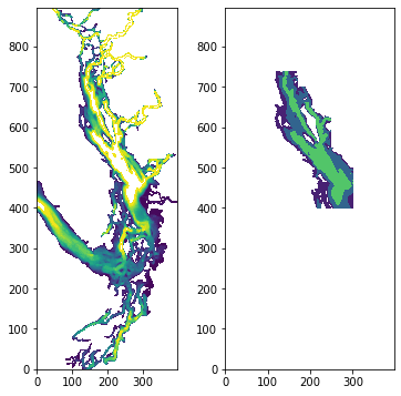
fig, ax = plt.subplots(1,2,figsize = (6,6))
with xr.open_dataset('/data/vdo/MEOPAR/NEMO-forcing/grid/bathymetry_201702.nc') as bathy:
bath=np.array(bathy.Bathymetry)
ax[0].contourf(bath,np.arange(0,250,10))
viz_tools.set_aspect(ax[0],coords='grid')
sogmask=np.copy(tmask[:,:,:,:])
sogmask[:,:,740:,:]=0
sogmask[:,:,700:,170:]=0
sogmask[:,:,550:,250:]=0
sogmask[:,:,:,302:]=0
sogmask[:,:,:400,:]=0
sogmask[:,:,:,:100]=0
#sogmask250[bath<250]=0
ax[1].contourf(np.ma.masked_where(sogmask[0,0,:,:]==0,bathy.Bathymetry),[0,100,250,550])
[4]:
<matplotlib.contour.QuadContourSet at 0x7f6540b14340>
[5]:
SMALL_SIZE = 15
MEDIUM_SIZE = 18
BIGGER_SIZE = 21

plt.rc('font', size=MEDIUM_SIZE)          # controls default text sizes
plt.rc('axes', titlesize=MEDIUM_SIZE)     # fontsize of the axes title
plt.rc('axes', labelsize=MEDIUM_SIZE)    # fontsize of the x and y labels
plt.rc('xtick', labelsize=MEDIUM_SIZE)    # fontsize of the tick labels
plt.rc('ytick', labelsize=MEDIUM_SIZE)    # fontsize of the tick labels
plt.rc('legend', fontsize=SMALL_SIZE)    # legend fontsize
plt.rc('figure', titlesize=BIGGER_SIZE)  # fontsize of the figure title
** Stop and check, have you made pickle files for all the years? **
[6]:
# loop through years of spring time series (mid feb-june) for bloom timing for 201905 run
years=list()
bloomtime1=list()
bloomtime2=list()
bloomtime3=list()
for year in range(startyear,endyear):
    fname3=f'springBloomTime_{str(year)}_{loc}_{modver}.pkl'
    savepath3=os.path.join(savedir,fname3)
    bio_time0,sno30,sdiat0,sflag0,scili0,diat_alld0,no3_alld0,flag_alld0,cili_alld0,phyto_alld0,\
                 intdiat0,intphyto0,fracdiat0,sphyto0,percdiat0=pickle.load(open(savepath3,'rb'))
    # put code that calculates bloom timing here
    bt1=bloomdrivers.metric1_bloomtime(phyto_alld0,no3_alld0,bio_time0)
    bt2=bloomdrivers.metric2_bloomtime(phyto_alld0,no3_alld0,bio_time0)
    bt3=bloomdrivers.metric3_bloomtime(sphyto0,sno30,bio_time0)
    years.append(year)
    bloomtime1.append(bt1)
    bloomtime2.append(bt2)
    bloomtime3.append(bt3)
years=np.array(years)
bloomtime1=np.array(bloomtime1)
bloomtime2=np.array(bloomtime2)
bloomtime3=np.array(bloomtime3)

# get year day
yearday1=et.datetimeToYD(bloomtime1)  # convert to year day tool
yearday2=et.datetimeToYD(bloomtime2)
yearday3=et.datetimeToYD(bloomtime3)
Combine separate year files into arrays:
[7]:
# loop through years (for location specific drivers)

years=list()
windjan=list()
windfeb=list()
windmar=list()
solarjan=list()
solarfeb=list()
solarmar=list()
parjan=list()
parfeb=list()
parmar=list()
tempjan=list()
tempfeb=list()
tempmar=list()
saljan=list()
salfeb=list()
salmar=list()
zoojan=list()
zoofeb=list()
zoomar=list()
mesozoojan=list()
mesozoofeb=list()
mesozoomar=list()
microzoojan=list()
microzoofeb=list()
microzoomar=list()
intzoojan=list()
intzoofeb=list()
intzoomar=list()
intmesozoojan=list()
intmesozoofeb=list()
intmesozoomar=list()
intmicrozoojan=list()
intmicrozoofeb=list()
intmicrozoomar=list()
midno3jan=list()
midno3feb=list()
midno3mar=list()

for year in range(startyear,endyear):
    fname=f'JanToMarch_TimeSeries_{year}_{loc}_{modver}.pkl'
    savepath=os.path.join(savedir,fname)
    bio_time,diat_alld,no3_alld,flag_alld,cili_alld,microzoo_alld,mesozoo_alld,\
            intdiat,intphyto,spar,intmesoz,intmicroz,grid_time,temp,salinity,u_wind,v_wind,twind,\
            solar,no3_30to90m,sno3,sdiat,sflag,scili,intzoop,fracdiat,zoop_alld,sphyto,phyto_alld,\
            percdiat,wspeed,winddirec=pickle.load(open(savepath,'rb'))
    # put code that calculates drivers here
    wind=bloomdrivers.D1_3monthly_avg(twind,wspeed)
    solar=bloomdrivers.D1_3monthly_avg(twind,solar)
    par=bloomdrivers.D1_3monthly_avg(bio_time,spar)
    temp=bloomdrivers.D1_3monthly_avg(grid_time,temp)
    sal=bloomdrivers.D1_3monthly_avg(grid_time,salinity)
    zoo=bloomdrivers.D2_3monthly_avg(bio_time,zoop_alld)
    mesozoo=bloomdrivers.D2_3monthly_avg(bio_time,mesozoo_alld)
    microzoo=bloomdrivers.D2_3monthly_avg(bio_time,microzoo_alld)
    intzoo=bloomdrivers.D1_3monthly_avg(bio_time,intzoop)
    intmesozoo=bloomdrivers.D1_3monthly_avg(bio_time,intmesoz)
    intmicrozoo=bloomdrivers.D1_3monthly_avg(bio_time,intmicroz)
    midno3=bloomdrivers.D1_3monthly_avg(bio_time,no3_30to90m)

    years.append(year)
    windjan.append(wind[0])
    windfeb.append(wind[1])
    windmar.append(wind[2])
    solarjan.append(solar[0])
    solarfeb.append(solar[1])
    solarmar.append(solar[2])
    parjan.append(par[0])
    parfeb.append(par[1])
    parmar.append(par[2])
    tempjan.append(temp[0])
    tempfeb.append(temp[1])
    tempmar.append(temp[2])
    saljan.append(sal[0])
    salfeb.append(sal[1])
    salmar.append(sal[2])
    zoojan.append(zoo[0])
    zoofeb.append(zoo[1])
    zoomar.append(zoo[2])
    mesozoojan.append(mesozoo[0])
    mesozoofeb.append(mesozoo[1])
    mesozoomar.append(mesozoo[2])
    microzoojan.append(microzoo[0])
    microzoofeb.append(microzoo[1])
    microzoomar.append(microzoo[2])
    intzoojan.append(intzoo[0])
    intzoofeb.append(intzoo[1])
    intzoomar.append(intzoo[2])
    intmesozoojan.append(intmesozoo[0])
    intmesozoofeb.append(intmesozoo[1])
    intmesozoomar.append(intmesozoo[2])
    intmicrozoojan.append(intmicrozoo[0])
    intmicrozoofeb.append(intmicrozoo[1])
    intmicrozoomar.append(intmicrozoo[2])
    midno3jan.append(midno3[0])
    midno3feb.append(midno3[1])
    midno3mar.append(midno3[2])

years=np.array(years)
windjan=np.array(windjan)
windfeb=np.array(windfeb)
windmar=np.array(windmar)
solarjan=np.array(solarjan)
solarfeb=np.array(solarfeb)
solarmar=np.array(solarmar)
parjan=np.array(parjan)
parfeb=np.array(parfeb)
parmar=np.array(parmar)
tempjan=np.array(tempjan)
tempfeb=np.array(tempfeb)
tempmar=np.array(tempmar)
saljan=np.array(saljan)
salfeb=np.array(salfeb)
salmar=np.array(salmar)
zoojan=np.array(zoojan)
zoofeb=np.array(zoofeb)
zoomar=np.array(zoomar)
mesozoojan=np.array(mesozoojan)
mesozoofeb=np.array(mesozoofeb)
mesozoomar=np.array(mesozoomar)
microzoojan=np.array(microzoojan)
microzoofeb=np.array(microzoofeb)
microzoomar=np.array(microzoomar)
intzoojan=np.array(intzoojan)
intzoofeb=np.array(intzoofeb)
intzoomar=np.array(intzoomar)
intmesozoojan=np.array(intmesozoojan)
intmesozoofeb=np.array(intmesozoofeb)
intmesozoomar=np.array(intmesozoomar)
intmicrozoojan=np.array(intmicrozoojan)
intmicrozoofeb=np.array(intmicrozoofeb)
intmicrozoomar=np.array(intmicrozoomar)
midno3jan=np.array(midno3jan)
midno3feb=np.array(midno3feb)
midno3mar=np.array(midno3mar)
[8]:
# loop through years (for non-location specific drivers)
fraserjan=list()
fraserfeb=list()
frasermar=list()
deepno3jan=list()
deepno3feb=list()
deepno3mar=list()

for year in range(startyear,endyear):
    fname2=f'JanToMarch_TimeSeries_{year}_{modver}.pkl'
    savepath2=os.path.join(savedir,fname2)
    no3_past250m,riv_time,rivFlow=pickle.load(open(savepath2,'rb'))
    # Code that calculates drivers here
    fraser=bloomdrivers.D1_3monthly_avg2(riv_time,rivFlow)
    fraserjan.append(fraser[0])
    fraserfeb.append(fraser[1])
    frasermar.append(fraser[2])

    fname=f'JanToMarch_TimeSeries_{year}_{loc}_{modver}.pkl'
    savepath=os.path.join(savedir,fname)
    bio_time,diat_alld,no3_alld,flag_alld,cili_alld,microzoo_alld,mesozoo_alld,\
            intdiat,intphyto,spar,intmesoz,intmicroz,grid_time,temp,salinity,u_wind,v_wind,twind,\
            solar,no3_30to90m,sno3,sdiat,sflag,scili,intzoop,fracdiat,zoop_alld,sphyto,phyto_alld,\
            percdiat,wspeed,winddirec=pickle.load(open(savepath,'rb'))
    deepno3=bloomdrivers.D1_3monthly_avg(bio_time,no3_past250m)

    deepno3jan.append(deepno3[0])
    deepno3feb.append(deepno3[1])
    deepno3mar.append(deepno3[2])

fraserjan=np.array(fraserjan)
fraserfeb=np.array(fraserfeb)
frasermar=np.array(frasermar)
deepno3jan=np.array(deepno3jan)
deepno3feb=np.array(deepno3feb)
deepno3mar=np.array(deepno3mar)
Load mixing variables
[9]:
# for T grid depth:
startd=dt.datetime(2015,1,1) # some date to get depth
endd=dt.datetime(2015,1,2)
basedir='/results2/SalishSea/nowcast-green.201905/'
nam_fmt='nowcast'
flen=1 # files contain 1 day of data each
tres=24 # 1: hourly resolution; 24: daily resolution
flist=et.index_model_files(startd,endd,basedir,nam_fmt,flen,"grid_T",tres)
with xr.open_mfdataset(flist['paths']) as gridt:
    depth_T=np.array(gridt.deptht)

# loop through years (for mixing drivers)

halojan=list()
halofeb=list()
halomar=list()
turbojan=list()
turbofeb=list()
turbomar=list()
densdiff5jan=list()
densdiff10jan=list()
densdiff15jan=list()
densdiff20jan=list()
densdiff25jan=list()
densdiff30jan=list()
densdiff5feb=list()
densdiff10feb=list()
densdiff15feb=list()
densdiff20feb=list()
densdiff25feb=list()
densdiff30feb=list()
densdiff5mar=list()
densdiff10mar=list()
densdiff15mar=list()
densdiff20mar=list()
densdiff25mar=list()
densdiff30mar=list()
eddy15jan=list()
eddy15feb=list()
eddy15mar=list()
eddy30jan=list()
eddy30feb=list()
eddy30mar=list()

for year in range(startyear,endyear):
    fname4=f'JanToMarch_Mixing_{year}_{loc}_{modver}.pkl'
    savepath4=os.path.join(savedir,fname4)
    halocline,eddy,depth,grid_time,temp,salinity=pickle.load(open(savepath4,'rb'))

    # halocline
    halo=bloomdrivers.D1_3monthly_avg(grid_time,halocline)
    halojan.append(halo[0])
    halofeb.append(halo[1])
    halomar.append(halo[2])
    # turbocline
    turbo=bloomdrivers.turbo(eddy,grid_time,depth_T)
    turbojan.append(turbo[0])
    turbofeb.append(turbo[1])
    turbomar.append(turbo[2])
    # density differences
    dict_diffs=bloomdrivers.density_diff(salinity,temp,grid_time)
    values=dict_diffs.values()
    all_diffs=list(values)
    densdiff5jan.append(all_diffs[0])
    densdiff10jan.append(all_diffs[3])
    densdiff15jan.append(all_diffs[6])
    densdiff20jan.append(all_diffs[9])
    densdiff25jan.append(all_diffs[12])
    densdiff30jan.append(all_diffs[15])
    densdiff5feb.append(all_diffs[1])
    densdiff10feb.append(all_diffs[4])
    densdiff15feb.append(all_diffs[7])
    densdiff20feb.append(all_diffs[10])
    densdiff25feb.append(all_diffs[13])
    densdiff30feb.append(all_diffs[16])
    densdiff5mar.append(all_diffs[2])
    densdiff10mar.append(all_diffs[5])
    densdiff15mar.append(all_diffs[8])
    densdiff20mar.append(all_diffs[11])
    densdiff25mar.append(all_diffs[14])
    densdiff30mar.append(all_diffs[17])
    # average eddy diffusivity
    avg_eddy=bloomdrivers.avg_eddy(eddy,grid_time,ij,ii)
    eddy15jan.append(avg_eddy[0])
    eddy15feb.append(avg_eddy[1])
    eddy15mar.append(avg_eddy[2])
    eddy30jan.append(avg_eddy[3])
    eddy30feb.append(avg_eddy[4])
    eddy30mar.append(avg_eddy[5])

halojan=np.array(halojan)
halofeb=np.array(halofeb)
halomar=np.array(halomar)
turbojan=np.array(turbojan)
turbofeb=np.array(turbofeb)
turbomar=np.array(turbomar)
densdiff5jan=np.array(densdiff5jan)
densdiff10jan=np.array(densdiff10jan)
densdiff15jan=np.array(densdiff15jan)
densdiff20jan=np.array(densdiff20jan)
densdiff25jan=np.array(densdiff25jan)
densdiff30jan=np.array(densdiff30jan)
densdiff5feb=np.array(densdiff5feb)
densdiff10feb=np.array(densdiff10feb)
densdiff15feb=np.array(densdiff15feb)
densdiff20feb=np.array(densdiff20feb)
densdiff25feb=np.array(densdiff25feb)
densdiff30feb=np.array(densdiff30feb)
densdiff5mar=np.array(densdiff5mar)
densdiff10mar=np.array(densdiff10mar)
densdiff15mar=np.array(densdiff15mar)
densdiff20mar=np.array(densdiff20mar)
densdiff25mar=np.array(densdiff25mar)
densdiff30mar=np.array(densdiff30mar)
eddy15jan=np.array(eddy15jan)
eddy15feb=np.array(eddy15feb)
eddy15mar=np.array(eddy15mar)
eddy30jan=np.array(eddy30jan)
eddy30feb=np.array(eddy30feb)
eddy30mar=np.array(eddy30mar)
[10]:
# January dataframe
dfjan=pd.DataFrame({'metric1':yearday1, 'metric2':yearday2, 'metric3':yearday3, 'wind':windjan,'solar':solarjan,
                  'temp':tempjan,'sal':saljan,'midno3':midno3jan,'fraser':fraserjan,'deepno3':deepno3jan,'halocline':halojan,
                   'turbocline':turbojan,'eddy15jan':eddy15jan,'eddy30jan':eddy30jan,'densdiff5jan':densdiff5jan,'densdiff10jan':densdiff10jan,
                    'densdiff15jan':densdiff15jan,'densdiff20jan':densdiff20jan,'densdiff25jan':densdiff25jan,'densdiff30jan':densdiff30jan})
# February dataframe
dffeb=pd.DataFrame({'metric1':yearday1, 'metric2':yearday2, 'metric3':yearday3, 'wind':windfeb,'solar':solarfeb,
                  'temp':tempfeb,'sal':salfeb,'midno3':midno3feb,'fraser':fraserfeb,'deepno3':deepno3feb,'halocline':halofeb,
                   'turbocline':turbofeb,'eddy15feb':eddy15feb,'eddy30feb':eddy30feb,'densdiff5feb':densdiff5feb,'densdiff10feb':densdiff10feb,
                    'densdiff15feb':densdiff15feb,'densdiff20feb':densdiff20feb,'densdiff25feb':densdiff25feb,'densdiff30feb':densdiff30feb})
# March dataframe
dfmar=pd.DataFrame({'Metric1':yearday1, 'Metric2':yearday2, 'Metric3':yearday3, 'Wind':windmar,'Solar':solarmar,
                  'Temp':tempmar,'Salinity':salmar,'Mid NO3':midno3mar,'Fraser':frasermar,'Deep NO3':deepno3mar,'Halocline':halomar,
                   'Turbocline':turbomar,'Eddy 15m':eddy15mar,'Eddy 30m':eddy30mar,'Dens diff 5m':densdiff5mar,'Dens diff 10m':densdiff10mar,
                    'Dens diff 15m':densdiff15mar,'Dens diff 20m':densdiff20mar,'Dens diff 25m':densdiff25mar,'Dens diff 30m':densdiff30mar})
[11]:
dfjan.cov()
[11]:
| metric1 | metric2 | metric3 | wind | solar | temp | sal | midno3 | fraser | deepno3 | halocline | turbocline | eddy15jan | eddy30jan | densdiff5jan | densdiff10jan | densdiff15jan | densdiff20jan | densdiff25jan | densdiff30jan | |
|---|---|---|---|---|---|---|---|---|---|---|---|---|---|---|---|---|---|---|---|---|
| metric1 | 167.192308 | 137.461538 | 128.192308 | 0.865513 | -12.446660 | -3.737684 | -2.507605 | 4.392353 | -600.550070 | 6.741225 | -13.428416 | -7.000595 | -0.016625 | -0.013287 | 0.660899 | 1.065900 | 1.024604 | 1.226255 | 1.324041 | 1.436117 |
| metric2 | 137.461538 | 180.571429 | 146.175824 | 4.023277 | -5.107036 | -5.014626 | -0.433000 | 5.376486 | -775.571390 | 7.828243 | -1.864832 | 1.989003 | 0.006909 | 0.000458 | -0.903692 | -0.690850 | -0.681681 | -0.466493 | -0.341531 | -0.186648 |
| metric3 | 128.192308 | 146.175824 | 132.335165 | 3.010450 | -8.356181 | -4.223339 | -1.419171 | 4.309779 | -801.435591 | 7.227635 | -4.460019 | 0.331795 | -0.001097 | -0.003846 | -0.404332 | 0.110955 | 0.193712 | 0.420024 | 0.537432 | 0.685603 |
| wind | 0.865513 | 4.023277 | 3.010450 | 0.870681 | -4.725488 | 0.097344 | 0.405484 | 0.267319 | -25.696723 | 0.225480 | 1.832783 | 1.971094 | 0.005867 | 0.003376 | -0.330454 | -0.336410 | -0.323170 | -0.313411 | -0.309029 | -0.299598 |
| solar | -12.446660 | -5.107036 | -8.356181 | -4.725488 | 67.435320 | -3.160387 | -2.825547 | -1.706040 | -23.614641 | -1.121300 | -10.159804 | -14.139872 | -0.039093 | -0.023628 | 1.603540 | 1.714917 | 1.721691 | 1.748888 | 1.795399 | 1.839209 |
| temp | -3.737684 | -5.014626 | -4.223339 | 0.097344 | -3.160387 | 0.487680 | 0.404520 | -0.077289 | 44.577452 | -0.310055 | 0.720811 | 0.740398 | 0.001745 | 0.001151 | -0.134744 | -0.220948 | -0.246962 | -0.267813 | -0.277333 | -0.286708 |
| sal | -2.507605 | -0.433000 | -1.419171 | 0.405484 | -2.825547 | 0.404520 | 0.863035 | 0.104467 | -18.401152 | -0.248327 | 1.601088 | 1.591486 | 0.003647 | 0.002234 | -0.351517 | -0.512916 | -0.566245 | -0.605198 | -0.618341 | -0.629426 |
| midno3 | 4.392353 | 5.376486 | 4.309779 | 0.267319 | -1.706040 | -0.077289 | 0.104467 | 0.570821 | -54.905988 | 0.519644 | 0.122078 | 0.321314 | 0.001469 | 0.000697 | -0.031115 | -0.027113 | -0.019738 | -0.017131 | -0.021077 | -0.025254 |
| fraser | -600.550070 | -775.571390 | -801.435591 | -25.696723 | -23.614641 | 44.577452 | -18.401152 | -54.905988 | 25704.091440 | -43.359271 | 3.227778 | -61.993284 | -0.032088 | -0.019895 | 5.228379 | -3.252128 | -4.681109 | -3.638878 | -2.685869 | -1.360753 |
| deepno3 | 6.741225 | 7.828243 | 7.227635 | 0.225480 | -1.121300 | -0.310055 | -0.248327 | 0.519644 | -43.359271 | 0.880773 | -0.338169 | -0.151289 | 0.000194 | -0.000173 | 0.028637 | 0.092383 | 0.123393 | 0.146730 | 0.151917 | 0.158164 |
| halocline | -13.428416 | -1.864832 | -4.460019 | 1.832783 | -10.159804 | 0.720811 | 1.601088 | 0.122078 | 3.227778 | -0.338169 | 6.064153 | 5.780585 | 0.015622 | 0.009495 | -0.921563 | -1.084373 | -1.106597 | -1.138140 | -1.145497 | -1.142760 |
| turbocline | -7.000595 | 1.989003 | 0.331795 | 1.971094 | -14.139872 | 0.740398 | 1.591486 | 0.321314 | -61.993284 | -0.151289 | 5.780585 | 6.190237 | 0.016168 | 0.009833 | -0.882268 | -0.997114 | -1.018206 | -1.050192 | -1.062436 | -1.067820 |
| eddy15jan | -0.016625 | 0.006909 | -0.001097 | 0.005867 | -0.039093 | 0.001745 | 0.003647 | 0.001469 | -0.032088 | 0.000194 | 0.015622 | 0.016168 | 0.000048 | 0.000029 | -0.002297 | -0.002466 | -0.002420 | -0.002428 | -0.002436 | -0.002421 |
| eddy30jan | -0.013287 | 0.000458 | -0.003846 | 0.003376 | -0.023628 | 0.001151 | 0.002234 | 0.000697 | -0.019895 | -0.000173 | 0.009495 | 0.009833 | 0.000029 | 0.000017 | -0.001355 | -0.001450 | -0.001424 | -0.001439 | -0.001449 | -0.001449 |
| densdiff5jan | 0.660899 | -0.903692 | -0.404332 | -0.330454 | 1.603540 | -0.134744 | -0.351517 | -0.031115 | 5.228379 | 0.028637 | -0.921563 | -0.882268 | -0.002297 | -0.001355 | 0.229026 | 0.278862 | 0.287768 | 0.293418 | 0.293281 | 0.290259 |
| densdiff10jan | 1.065900 | -0.690850 | 0.110955 | -0.336410 | 1.714917 | -0.220948 | -0.512916 | -0.027113 | -3.252128 | 0.092383 | -1.084373 | -0.997114 | -0.002466 | -0.001450 | 0.278862 | 0.378338 | 0.405244 | 0.420971 | 0.423704 | 0.422999 |
| densdiff15jan | 1.024604 | -0.681681 | 0.193712 | -0.323170 | 1.721691 | -0.246962 | -0.566245 | -0.019738 | -4.681109 | 0.123393 | -1.106597 | -1.018206 | -0.002420 | -0.001424 | 0.287768 | 0.405244 | 0.440322 | 0.460498 | 0.464472 | 0.464913 |
| densdiff20jan | 1.226255 | -0.466493 | 0.420024 | -0.313411 | 1.748888 | -0.267813 | -0.605198 | -0.017131 | -3.638878 | 0.146730 | -1.138140 | -1.050192 | -0.002428 | -0.001439 | 0.293418 | 0.420971 | 0.460498 | 0.484052 | 0.489341 | 0.491269 |
| densdiff25jan | 1.324041 | -0.341531 | 0.537432 | -0.309029 | 1.795399 | -0.277333 | -0.618341 | -0.021077 | -2.685869 | 0.151917 | -1.145497 | -1.062436 | -0.002436 | -0.001449 | 0.293281 | 0.423704 | 0.464472 | 0.489341 | 0.495359 | 0.498217 |
| densdiff30jan | 1.436117 | -0.186648 | 0.685603 | -0.299598 | 1.839209 | -0.286708 | -0.629426 | -0.025254 | -1.360753 | 0.158164 | -1.142760 | -1.067820 | -0.002421 | -0.001449 | 0.290259 | 0.422999 | 0.464913 | 0.491269 | 0.498217 | 0.502352 |
[12]:
dffeb.cov()
[12]:
| metric1 | metric2 | metric3 | wind | solar | temp | sal | midno3 | fraser | deepno3 | halocline | turbocline | eddy15feb | eddy30feb | densdiff5feb | densdiff10feb | densdiff15feb | densdiff20feb | densdiff25feb | densdiff30feb | |
|---|---|---|---|---|---|---|---|---|---|---|---|---|---|---|---|---|---|---|---|---|
| metric1 | 167.192308 | 137.461538 | 128.192308 | 3.177590 | -53.858452 | -0.713898 | -4.898713 | 3.904678 | -939.299268 | 6.694636 | -4.389741 | 0.554748 | 0.014635 | 0.007819 | 2.383530 | 3.761208 | 3.909286 | 3.847092 | 3.887294 | 3.985908 |
| metric2 | 137.461538 | 180.571429 | 146.175824 | 4.287622 | -27.990300 | -6.175048 | -4.867767 | 4.396219 | -2191.031450 | 7.704300 | 0.937233 | 4.748586 | 0.023554 | 0.012652 | 1.897252 | 3.612524 | 3.928376 | 3.909006 | 3.945590 | 3.989792 |
| metric3 | 128.192308 | 146.175824 | 132.335165 | 3.445910 | -37.739568 | -4.270886 | -5.689764 | 3.862083 | -1862.155986 | 7.144473 | 0.061211 | 1.754537 | 0.015185 | 0.008215 | 1.965924 | 3.684893 | 4.123033 | 4.231658 | 4.305993 | 4.420662 |
| wind | 3.177590 | 4.287622 | 3.445910 | 0.301236 | -1.559052 | -0.141542 | 0.200360 | 0.121171 | -73.324974 | 0.170992 | 0.643850 | 0.851012 | 0.002127 | 0.001137 | -0.152347 | -0.196612 | -0.194572 | -0.187359 | -0.182976 | -0.178600 |
| solar | -53.858452 | -27.990300 | -37.739568 | -1.559052 | 58.542495 | -0.877576 | 2.507346 | -1.635060 | 240.859673 | -3.642172 | 1.174798 | 0.497177 | -0.006591 | -0.003214 | -0.974991 | -1.633321 | -1.783844 | -1.923382 | -1.958474 | -2.013415 |
| temp | -0.713898 | -6.175048 | -4.270886 | -0.141542 | -0.877576 | 0.714746 | 0.317722 | -0.152104 | 183.593070 | -0.308140 | -0.157110 | -0.055253 | -0.000120 | -0.000024 | -0.063457 | -0.203240 | -0.249643 | -0.260430 | -0.264205 | -0.265582 |
| sal | -4.898713 | -4.867767 | -5.689764 | 0.200360 | 2.507346 | 0.317722 | 1.535570 | 0.018919 | -60.189150 | -0.645027 | 1.301662 | 1.953059 | 0.003289 | 0.001779 | -0.621843 | -1.004808 | -1.111158 | -1.147287 | -1.154864 | -1.165371 |
| midno3 | 3.904678 | 4.396219 | 3.862083 | 0.121171 | -1.635060 | -0.152104 | 0.018919 | 0.473593 | -161.052481 | 0.426217 | -0.012849 | 0.375524 | 0.001098 | 0.000633 | 0.108866 | 0.099354 | 0.059863 | 0.043926 | 0.041519 | 0.040145 |
| fraser | -939.299268 | -2191.031450 | -1862.155986 | -73.324974 | 240.859673 | 183.593070 | -60.189150 | -161.052481 | 122323.912955 | -76.481005 | -134.642912 | -252.651984 | -0.445890 | -0.236513 | 7.861906 | 8.799545 | 12.802585 | 16.051097 | 15.993412 | 15.701236 |
| deepno3 | 6.694636 | 7.704300 | 7.144473 | 0.170992 | -3.642172 | -0.308140 | -0.645027 | 0.426217 | -76.481005 | 0.869508 | -0.216816 | -0.187361 | 0.000629 | 0.000366 | 0.289162 | 0.451036 | 0.468765 | 0.480905 | 0.485948 | 0.492192 |
| halocline | -4.389741 | 0.937233 | 0.061211 | 0.643850 | 1.174798 | -0.157110 | 1.301662 | -0.012849 | -134.642912 | -0.216816 | 3.082319 | 3.095604 | 0.006061 | 0.003350 | -0.818087 | -1.132523 | -1.153252 | -1.126900 | -1.115023 | -1.107319 |
| turbocline | 0.554748 | 4.748586 | 1.754537 | 0.851012 | 0.497177 | -0.055253 | 1.953059 | 0.375524 | -252.651984 | -0.187361 | 3.095604 | 4.193016 | 0.008477 | 0.004649 | -0.892831 | -1.389728 | -1.500802 | -1.517380 | -1.514614 | -1.516796 |
| eddy15feb | 0.014635 | 0.023554 | 0.015185 | 0.002127 | -0.006591 | -0.000120 | 0.003289 | 0.001098 | -0.445890 | 0.000629 | 0.006061 | 0.008477 | 0.000020 | 0.000011 | -0.001484 | -0.002367 | -0.002609 | -0.002652 | -0.002649 | -0.002654 |
| eddy30feb | 0.007819 | 0.012652 | 0.008215 | 0.001137 | -0.003214 | -0.000024 | 0.001779 | 0.000633 | -0.236513 | 0.000366 | 0.003350 | 0.004649 | 0.000011 | 0.000006 | -0.000775 | -0.001267 | -0.001406 | -0.001432 | -0.001431 | -0.001435 |
| densdiff5feb | 2.383530 | 1.897252 | 1.965924 | -0.152347 | -0.974991 | -0.063457 | -0.621843 | 0.108866 | 7.861906 | 0.289162 | -0.818087 | -0.892831 | -0.001484 | -0.000775 | 0.366259 | 0.504221 | 0.516901 | 0.514668 | 0.512305 | 0.510859 |
| densdiff10feb | 3.761208 | 3.612524 | 3.684893 | -0.196612 | -1.633321 | -0.203240 | -1.004808 | 0.099354 | 8.799545 | 0.451036 | -1.132523 | -1.389728 | -0.002367 | -0.001267 | 0.504221 | 0.761475 | 0.808103 | 0.815463 | 0.814916 | 0.815031 |
| densdiff15feb | 3.909286 | 3.928376 | 4.123033 | -0.194572 | -1.783844 | -0.249643 | -1.111158 | 0.059863 | 12.802585 | 0.468765 | -1.153252 | -1.500802 | -0.002609 | -0.001406 | 0.516901 | 0.808103 | 0.873965 | 0.889659 | 0.891100 | 0.893135 |
| densdiff20feb | 3.847092 | 3.909006 | 4.231658 | -0.187359 | -1.923382 | -0.260430 | -1.147287 | 0.043926 | 16.051097 | 0.480905 | -1.126900 | -1.517380 | -0.002652 | -0.001432 | 0.514668 | 0.815463 | 0.889659 | 0.910435 | 0.913174 | 0.916506 |
| densdiff25feb | 3.887294 | 3.945590 | 4.305993 | -0.182976 | -1.958474 | -0.264205 | -1.154864 | 0.041519 | 15.993412 | 0.485948 | -1.115023 | -1.514614 | -0.002649 | -0.001431 | 0.512305 | 0.814916 | 0.891100 | 0.913174 | 0.916360 | 0.920232 |
| densdiff30feb | 3.985908 | 3.989792 | 4.420662 | -0.178600 | -2.013415 | -0.265582 | -1.165371 | 0.040145 | 15.701236 | 0.492192 | -1.107319 | -1.516796 | -0.002654 | -0.001435 | 0.510859 | 0.815031 | 0.893135 | 0.916506 | 0.920232 | 0.924942 |
[13]:
dfmar.cov()
[13]:
| Metric1 | Metric2 | Metric3 | Wind | Solar | Temp | Salinity | Mid NO3 | Fraser | Deep NO3 | Halocline | Turbocline | Eddy 15m | Eddy 30m | Dens diff 5m | Dens diff 10m | Dens diff 15m | Dens diff 20m | Dens diff 25m | Dens diff 30m | |
|---|---|---|---|---|---|---|---|---|---|---|---|---|---|---|---|---|---|---|---|---|
| Metric1 | 167.192308 | 137.461538 | 128.192308 | 8.754072 | -182.929908 | -2.243489 | 4.867424 | 5.951665 | -850.715675 | 6.772832 | 12.937388 | 20.499302 | 0.046715 | 0.025753 | -3.070548 | -4.896818 | -5.058046 | -4.947842 | -4.897806 | -4.840299 |
| Metric2 | 137.461538 | 180.571429 | 146.175824 | 9.077360 | -180.540067 | -6.788121 | 5.232388 | 7.160443 | -3250.417519 | 7.694176 | 13.315534 | 21.953639 | 0.053338 | 0.029672 | -3.136544 | -4.486028 | -4.891891 | -4.866103 | -4.819508 | -4.774288 |
| Metric3 | 128.192308 | 146.175824 | 132.335165 | 7.854858 | -163.303261 | -4.494384 | 4.504952 | 6.459397 | -2129.210389 | 7.127748 | 11.296432 | 19.263727 | 0.046704 | 0.025858 | -2.640806 | -4.001602 | -4.341096 | -4.320247 | -4.280629 | -4.238613 |
| Wind | 8.754072 | 9.077360 | 7.854858 | 0.745308 | -14.003825 | -0.218967 | 0.412653 | 0.429244 | -29.919179 | 0.495395 | 1.512662 | 1.783337 | 0.004730 | 0.002612 | -0.241697 | -0.367929 | -0.410721 | -0.409620 | -0.404859 | -0.399256 |
| Solar | -182.929908 | -180.540067 | -163.303261 | -14.003825 | 401.115077 | 2.802207 | -6.910096 | -5.339316 | -1722.072976 | -8.563671 | -19.872191 | -30.512211 | -0.070921 | -0.039276 | 4.376455 | 6.205914 | 7.207849 | 7.407072 | 7.353046 | 7.291933 |
| Temp | -2.243489 | -6.788121 | -4.494384 | -0.218967 | 2.802207 | 0.460763 | -0.076910 | -0.322029 | 238.741716 | -0.324212 | -0.253645 | -0.509576 | -0.001541 | -0.000872 | 0.027931 | 0.024538 | 0.040026 | 0.041684 | 0.041229 | 0.041877 |
| Salinity | 4.867424 | 5.232388 | 4.504952 | 0.412653 | -6.910096 | -0.076910 | 0.896922 | 0.248659 | -169.872150 | -0.129176 | 1.876504 | 1.437821 | 0.003553 | 0.002003 | -0.455622 | -0.706000 | -0.773812 | -0.773844 | -0.769913 | -0.761883 |
| Mid NO3 | 5.951665 | 7.160443 | 6.459397 | 0.429244 | -5.339316 | -0.322029 | 0.248659 | 0.673588 | -229.004563 | 0.527731 | 0.807674 | 1.066004 | 0.003202 | 0.001763 | -0.124549 | -0.184844 | -0.199858 | -0.189961 | -0.184451 | -0.177915 |
| Fraser | -850.715675 | -3250.417519 | -2129.210389 | -29.919179 | -1722.072976 | 238.741716 | -169.872150 | -229.004563 | 234451.617848 | -54.719142 | -126.928343 | -189.118196 | -0.516486 | -0.286979 | 75.990121 | 98.572787 | 102.095629 | 97.690653 | 96.936242 | 96.272999 |
| Deep NO3 | 6.772832 | 7.694176 | 7.127748 | 0.495395 | -8.563671 | -0.324212 | -0.129176 | 0.527731 | -54.719142 | 0.853843 | 0.670977 | 1.046770 | 0.003425 | 0.001934 | 0.056219 | 0.085238 | 0.077538 | 0.068121 | 0.066951 | 0.065363 |
| Halocline | 12.937388 | 13.315534 | 11.296432 | 1.512662 | -19.872191 | -0.253645 | 1.876504 | 0.807674 | -126.928343 | 0.670977 | 7.817049 | 5.010816 | 0.015494 | 0.009034 | -0.949263 | -1.596961 | -1.817484 | -1.862745 | -1.859846 | -1.838261 |
| Turbocline | 20.499302 | 21.953639 | 19.263727 | 1.783337 | -30.512211 | -0.509576 | 1.437821 | 1.066004 | -189.118196 | 1.046770 | 5.010816 | 4.882223 | 0.013393 | 0.007537 | -0.810031 | -1.270334 | -1.410447 | -1.413311 | -1.401348 | -1.381726 |
| Eddy 15m | 0.046715 | 0.053338 | 0.046704 | 0.004730 | -0.070921 | -0.001541 | 0.003553 | 0.003202 | -0.516486 | 0.003425 | 0.015494 | 0.013393 | 0.000040 | 0.000023 | -0.001903 | -0.003120 | -0.003560 | -0.003603 | -0.003577 | -0.003526 |
| Eddy 30m | 0.025753 | 0.029672 | 0.025858 | 0.002612 | -0.039276 | -0.000872 | 0.002003 | 0.001763 | -0.286979 | 0.001934 | 0.009034 | 0.007537 | 0.000023 | 0.000013 | -0.001068 | -0.001771 | -0.002029 | -0.002061 | -0.002048 | -0.002020 |
| Dens diff 5m | -3.070548 | -3.136544 | -2.640806 | -0.241697 | 4.376455 | 0.027931 | -0.455622 | -0.124549 | 75.990121 | 0.056219 | -0.949263 | -0.810031 | -0.001903 | -0.001068 | 0.252805 | 0.376863 | 0.405617 | 0.402980 | 0.399861 | 0.394240 |
| Dens diff 10m | -4.896818 | -4.486028 | -4.001602 | -0.367929 | 6.205914 | 0.024538 | -0.706000 | -0.184844 | 98.572787 | 0.085238 | -1.596961 | -1.270334 | -0.003120 | -0.001771 | 0.376863 | 0.596848 | 0.646302 | 0.641576 | 0.636498 | 0.627298 |
| Dens diff 15m | -5.058046 | -4.891891 | -4.341096 | -0.410721 | 7.207849 | 0.040026 | -0.773812 | -0.199858 | 102.095629 | 0.077538 | -1.817484 | -1.410447 | -0.003560 | -0.002029 | 0.405617 | 0.646302 | 0.707221 | 0.705481 | 0.700609 | 0.691254 |
| Dens diff 20m | -4.947842 | -4.866103 | -4.320247 | -0.409620 | 7.407072 | 0.041684 | -0.773844 | -0.189961 | 97.690653 | 0.068121 | -1.862745 | -1.413311 | -0.003603 | -0.002061 | 0.402980 | 0.641576 | 0.705481 | 0.706935 | 0.702976 | 0.694443 |
| Dens diff 25m | -4.897806 | -4.819508 | -4.280629 | -0.404859 | 7.353046 | 0.041229 | -0.769913 | -0.184451 | 96.936242 | 0.066951 | -1.859846 | -1.401348 | -0.003577 | -0.002048 | 0.399861 | 0.636498 | 0.700609 | 0.702976 | 0.699391 | 0.691274 |
| Dens diff 30m | -4.840299 | -4.774288 | -4.238613 | -0.399256 | 7.291933 | 0.041877 | -0.761883 | -0.177915 | 96.272999 | 0.065363 | -1.838261 | -1.381726 | -0.003526 | -0.002020 | 0.394240 | 0.627298 | 0.691254 | 0.694443 | 0.691274 | 0.683730 |
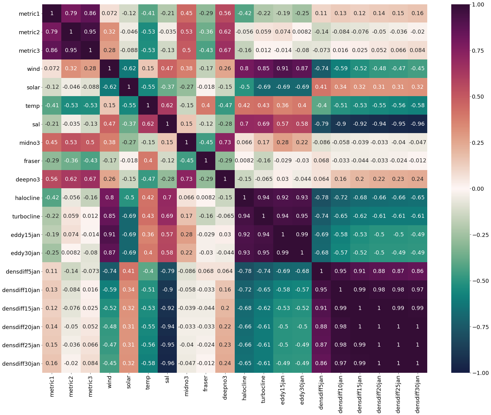
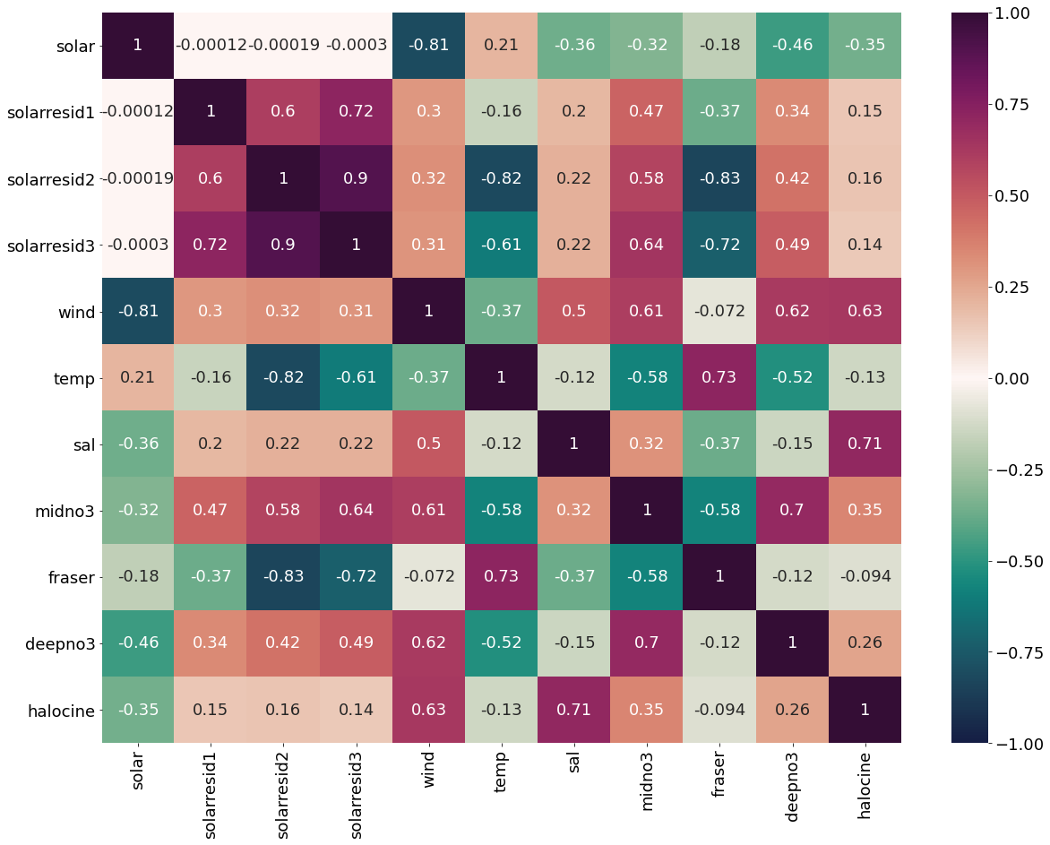
Correlation matrix for January Values
[14]:
plt.subplots(figsize=(28,22))
cm1=cmocean.cm.curl
sns.heatmap(dfjan.corr(), annot = True,cmap=cm1,vmin=-1,vmax=1)
[14]:
<AxesSubplot:>
Correlation matrix for February Values
[15]:
plt.subplots(figsize=(28,22))
cm1=cmocean.cm.curl
sns.heatmap(dffeb.corr(), annot = True,cmap=cm1,vmin=-1,vmax=1)
[15]:
<AxesSubplot:>
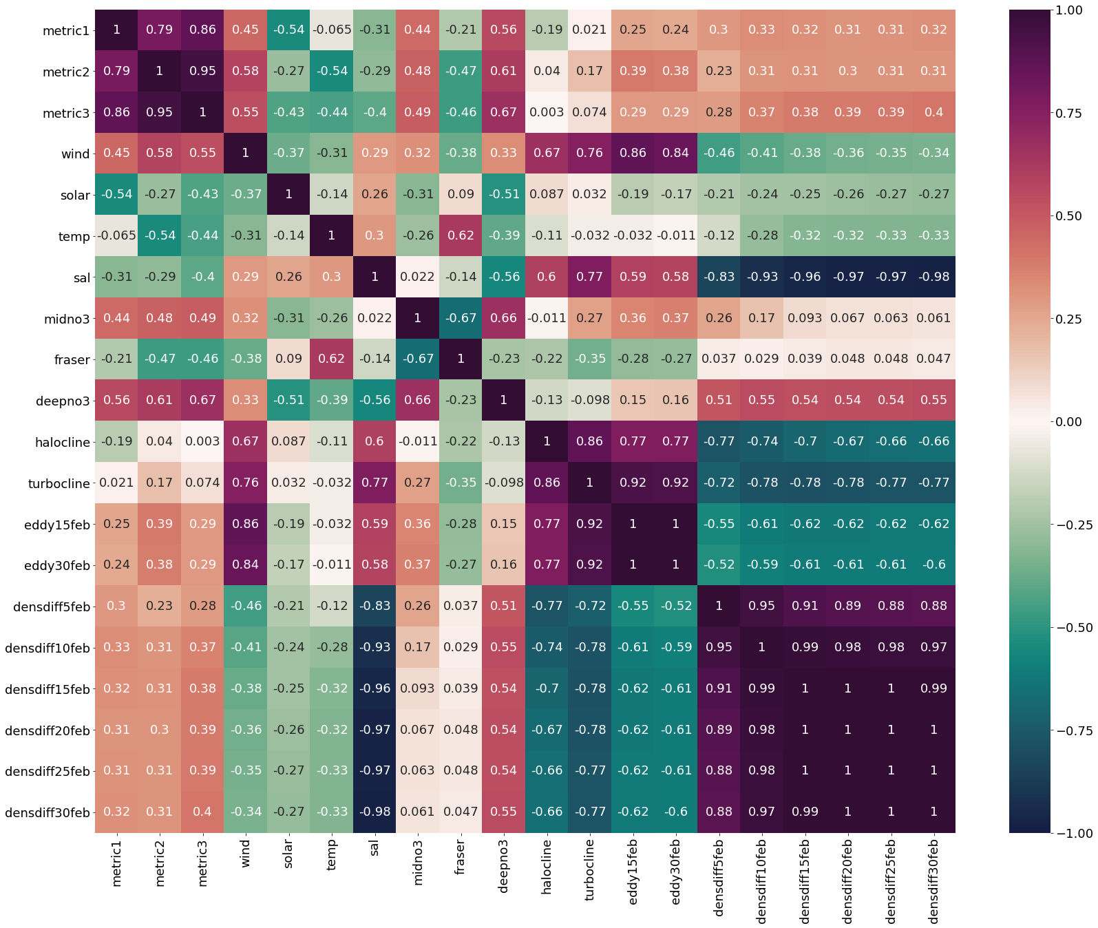
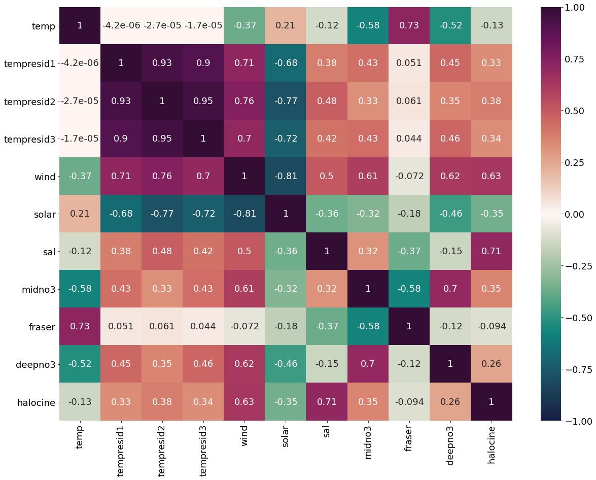
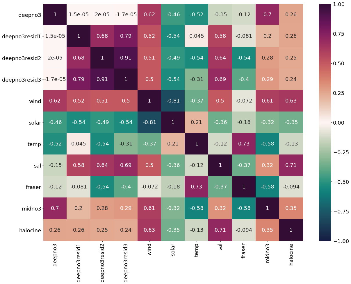
Correlation matrix for March Values
[16]:
plt.subplots(figsize=(28,22))
cm1=cmocean.cm.curl
marchheat=sns.heatmap(dffeb.corr(), annot = True,cmap=cm1,vmin=-1,vmax=1)
fig=marchheat.get_figure()
#fig.savefig('/ocean/aisabell/MEOPAR/report_figures/S3march_correlations.png',dpi=300)

Correlation plots of wind residuals
[17]:
# Wind residual calculations for each metric
windresid1=list()
y,r2,m,b=bloomdrivers.reg_r2(windmar,yearday1)
for ind,y in enumerate(yearday1):
    x=windmar[ind]
    windresid1.append(y-(m*x+b))

windresid2=list()
y,r2,m,b=bloomdrivers.reg_r2(windmar,yearday2)
for ind,y in enumerate(yearday2):
    x=windmar[ind]
    windresid2.append(y-(m*x+b))

windresid3=list()
y,r2,m,b=bloomdrivers.reg_r2(windmar,yearday3)
for ind,y in enumerate(yearday3):
    x=windmar[ind]
    windresid3.append(y-(m*x+b))
[18]:
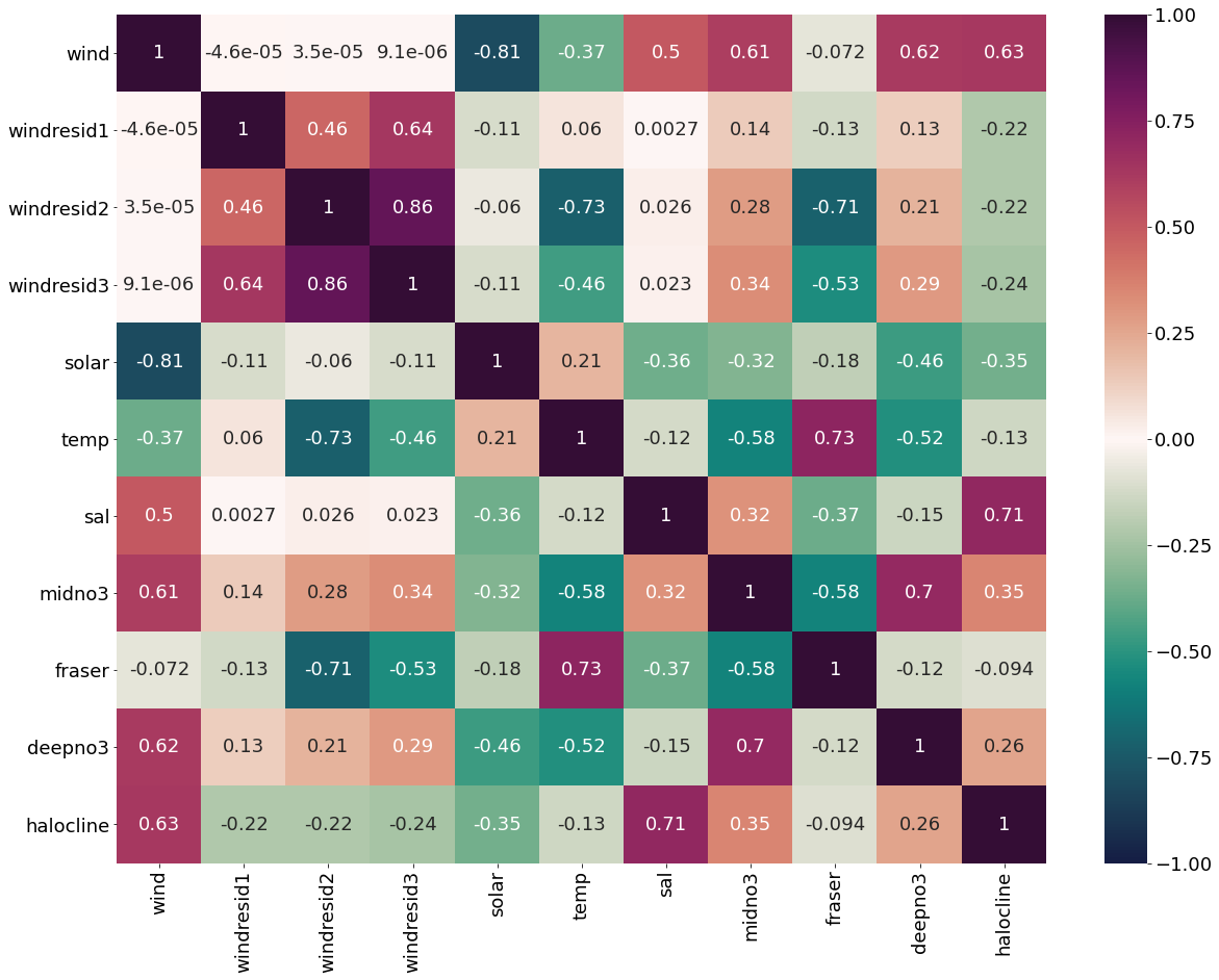
dfwind=pd.DataFrame({'wind':windmar,'windresid1':windresid1,'windresid2':windresid2,'windresid3':windresid3,'solar':solarmar,
                  'temp':tempmar,'sal':salmar,'midno3':midno3mar,'fraser':frasermar,'deepno3':deepno3mar,'halocline':halomar})
[19]:
plt.subplots(figsize=(20,15))
cm1=cmocean.cm.curl
sns.heatmap(dfwind.corr(), annot = True,cmap=cm1,vmin=-1,vmax=1)
[19]:
<AxesSubplot:>
[20]:
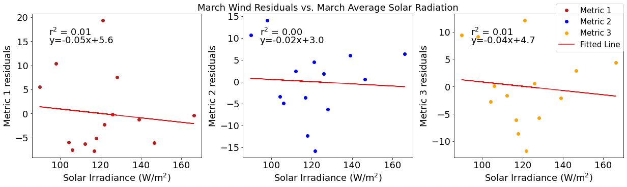
# ---------- Solar ---------
fig4,ax4=plt.subplots(1,3,figsize=(17,5),constrained_layout=True)
ax4[0].plot(solarmar,windresid1,'o',color='firebrick',label='Metric 1')
ax4[0].set_xlabel('Solar Irradiance (W/$\mathregular{m^2}$)')
ax4[0].set_ylabel('Metric 1 residuals')
y,r2,m,b=bloomdrivers.reg_r2(solarmar,windresid1)
ax4[0].plot(solarmar, y, 'r')
ax4[0].text(0.1, 0.85, '$\mathregular{r^2}$ = %.2f'%r2, transform=ax4[0].transAxes)
ax4[0].text(0.1,0.78,f'y={round(m,2)}x+{round(b,1)}',horizontalalignment='left',verticalalignment='bottom',transform=ax4[0].transAxes)

ax4[1].plot(solarmar,windresid2,'o',color='b',label='Metric 2')
ax4[1].set_xlabel('Solar Irradiance (W/$\mathregular{m^2}$)')
ax4[1].set_ylabel('Metric 2 residuals')
ax4[1].set_title('March Wind Residuals vs. March Average Solar Radiation')
y,r2,m,b=bloomdrivers.reg_r2(solarmar,windresid2)
ax4[1].plot(solarmar, y, 'r')
ax4[1].text(0.1, 0.85, '$\mathregular{r^2}$ = %.2f'%r2, transform=ax4[1].transAxes)
ax4[1].text(0.1,0.78,f'y={round(m,2)}x+{round(b,1)}',horizontalalignment='left',verticalalignment='bottom',transform=ax4[1].transAxes)

ax4[2].plot(solarmar,windresid3,'o',color='orange',label='Metric 3')
ax4[2].set_xlabel('Solar Irradiance (W/$\mathregular{m^2}$)')
ax4[2].set_ylabel('Metric 3 residuals')
y,r2,m,b=bloomdrivers.reg_r2(solarmar,windresid3)
ax4[2].plot(solarmar, y, 'r', label='Fitted Line')
ax4[2].text(0.1, 0.85, '$\mathregular{r^2}$ = %.2f'%r2, transform=ax4[2].transAxes)
ax4[2].text(0.1,0.78,f'y={round(m,2)}x+{round(b,1)}',horizontalalignment='left',verticalalignment='bottom',transform=ax4[2].transAxes)
fig4.legend()
[20]:
<matplotlib.legend.Legend at 0x7f652b489b80>
[21]:
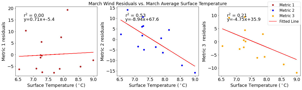
# ---------- Temperature ---------
fig4,ax4=plt.subplots(1,3,figsize=(17,5),constrained_layout=True)
ax4[0].plot(tempmar,windresid1,'o',color='firebrick',label='Metric 1')
ax4[0].set_xlabel('Surface Temperature ($^\circ$C)')
ax4[0].set_ylabel('Metric 1 residuals')
y,r2,m,b=bloomdrivers.reg_r2(tempmar,windresid1)
ax4[0].plot(tempmar, y, 'r')
ax4[0].text(0.1, 0.85, '$\mathregular{r^2}$ = %.2f'%r2, transform=ax4[0].transAxes)
ax4[0].text(0.1,0.78,f'y={round(m,2)}x+{round(b,1)}',horizontalalignment='left',verticalalignment='bottom',transform=ax4[0].transAxes)

ax4[1].plot(tempmar,windresid2,'o',color='b',label='Metric 2')
ax4[1].set_xlabel('Surface Temperature ($^\circ$C)')
ax4[1].set_ylabel('Metric 2 residuals')
ax4[1].set_title('March Wind Residuals vs. March Average Surface Temperature')
y,r2,m,b=bloomdrivers.reg_r2(tempmar,windresid2)
ax4[1].plot(tempmar, y, 'r')
ax4[1].text(0.1, 0.85, '$\mathregular{r^2}$ = %.2f'%r2, transform=ax4[1].transAxes)
ax4[1].text(0.1,0.78,f'y={round(m,2)}x+{round(b,1)}',horizontalalignment='left',verticalalignment='bottom',transform=ax4[1].transAxes)

ax4[2].plot(tempmar,windresid3,'o',color='orange',label='Metric 3')
ax4[2].set_xlabel('Surface Temperature ($^\circ$C)')
ax4[2].set_ylabel('Metric 3  residuals')
y,r2,m,b=bloomdrivers.reg_r2(tempmar,windresid3)
ax4[2].plot(tempmar, y, 'r', label='Fitted Line')
ax4[2].text(0.1, 0.85, '$\mathregular{r^2}$ = %.2f'%r2, transform=ax4[2].transAxes)
ax4[2].text(0.1,0.78,f'y={round(m,2)}x+{round(b,1)}',horizontalalignment='left',verticalalignment='bottom',transform=ax4[2].transAxes)
fig4.legend()
[21]:
<matplotlib.legend.Legend at 0x7f652b365bb0>
[22]:
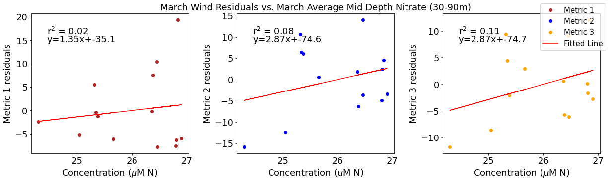
# ---------- Mid NO3 ---------
fig4,ax4=plt.subplots(1,3,figsize=(17,5),constrained_layout=True)
ax4[0].plot(midno3mar,windresid1,'o',color='firebrick',label='Metric 1')
ax4[0].set_xlabel('Concentration ($\mu$M N)')
ax4[0].set_ylabel('Metric 1 residuals')
y,r2,m,b=bloomdrivers.reg_r2(midno3mar,windresid1)
ax4[0].plot(midno3mar, y, 'r')
ax4[0].text(0.1, 0.85, '$\mathregular{r^2}$ = %.2f'%r2, transform=ax4[0].transAxes)
ax4[0].text(0.1,0.78,f'y={round(m,2)}x+{round(b,1)}',horizontalalignment='left',verticalalignment='bottom',transform=ax4[0].transAxes)

ax4[1].plot(midno3mar,windresid2,'o',color='b',label='Metric 2')
ax4[1].set_xlabel('Concentration ($\mu$M N)')
ax4[1].set_ylabel('Metric 2 residuals')
ax4[1].set_title('March Wind Residuals vs. March Average Mid Depth Nitrate (30-90m)')
y,r2,m,b=bloomdrivers.reg_r2(midno3mar,windresid2)
ax4[1].plot(midno3mar, y, 'r')
ax4[1].text(0.1, 0.85, '$\mathregular{r^2}$ = %.2f'%r2, transform=ax4[1].transAxes)
ax4[1].text(0.1,0.78,f'y={round(m,2)}x+{round(b,1)}',horizontalalignment='left',verticalalignment='bottom',transform=ax4[1].transAxes)

ax4[2].plot(midno3mar,windresid3,'o',color='orange',label='Metric 3')
ax4[2].set_xlabel('Concentration ($\mu$M N)')
ax4[2].set_ylabel('Metric 3 residuals')
y,r2,m,b=bloomdrivers.reg_r2(midno3mar,windresid3)
ax4[2].plot(midno3mar, y, 'r', label='Fitted Line')
ax4[2].text(0.1, 0.85, '$\mathregular{r^2}$ = %.2f'%r2, transform=ax4[2].transAxes)
ax4[2].text(0.1,0.78,f'y={round(m,2)}x+{round(b,1)}',horizontalalignment='left',verticalalignment='bottom',transform=ax4[2].transAxes)
fig4.legend()
[22]:
<matplotlib.legend.Legend at 0x7f652b227910>
[23]:
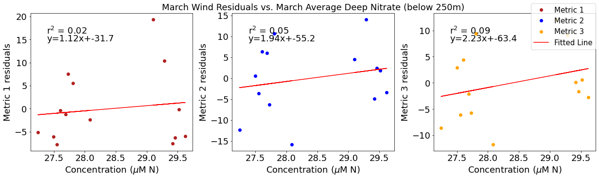
# ---------- Deep NO3 ---------
fig4,ax4=plt.subplots(1,3,figsize=(17,5),constrained_layout=True)
ax4[0].plot(deepno3mar,windresid1,'o',color='firebrick',label='Metric 1')
ax4[0].set_xlabel('Concentration ($\mu$M N)')
ax4[0].set_ylabel('Metric 1 residuals')
y,r2,m,b=bloomdrivers.reg_r2(deepno3mar,windresid1)
ax4[0].plot(deepno3mar, y, 'r')
ax4[0].text(0.1, 0.85, '$\mathregular{r^2}$ = %.2f'%r2, transform=ax4[0].transAxes)
ax4[0].text(0.1,0.78,f'y={round(m,2)}x+{round(b,1)}',horizontalalignment='left',verticalalignment='bottom',transform=ax4[0].transAxes)

ax4[1].plot(deepno3mar,windresid2,'o',color='b',label='Metric 2')
ax4[1].set_xlabel('Concentration ($\mu$M N)')
ax4[1].set_ylabel('Metric 2 residuals')
ax4[1].set_title('March Wind Residuals vs. March Average Deep Nitrate (below 250m)')
y,r2,m,b=bloomdrivers.reg_r2(deepno3mar,windresid2)
ax4[1].plot(deepno3mar, y, 'r')
ax4[1].text(0.1, 0.85, '$\mathregular{r^2}$ = %.2f'%r2, transform=ax4[1].transAxes)
ax4[1].text(0.1,0.78,f'y={round(m,2)}x+{round(b,1)}',horizontalalignment='left',verticalalignment='bottom',transform=ax4[1].transAxes)

ax4[2].plot(deepno3mar,windresid3,'o',color='orange',label='Metric 3')
ax4[2].set_xlabel('Concentration ($\mu$M N)')
ax4[2].set_ylabel('Metric 3 residuals')
y,r2,m,b=bloomdrivers.reg_r2(deepno3mar,windresid3)
ax4[2].plot(deepno3mar, y, 'r', label='Fitted Line')
ax4[2].text(0.1, 0.85, '$\mathregular{r^2}$ = %.2f'%r2, transform=ax4[2].transAxes)
ax4[2].text(0.1,0.78,f'y={round(m,2)}x+{round(b,1)}',horizontalalignment='left',verticalalignment='bottom',transform=ax4[2].transAxes)
fig4.legend()
[23]:
<matplotlib.legend.Legend at 0x7f652b0d9e50>
[24]:
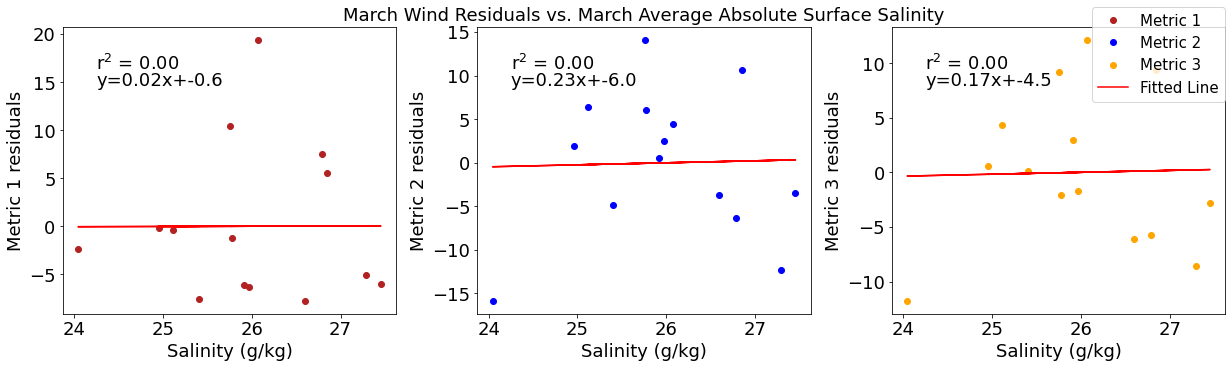
# ---------- Salinity ---------
fig4,ax4=plt.subplots(1,3,figsize=(17,5),constrained_layout=True)
ax4[0].plot(salmar,windresid1,'o',color='firebrick',label='Metric 1')
ax4[0].set_xlabel('Salinity (g/kg)')
ax4[0].set_ylabel('Metric 1 residuals')
y,r2,m,b=bloomdrivers.reg_r2(salmar,windresid1)
ax4[0].plot(salmar, y, 'r')
ax4[0].text(0.1, 0.85, '$\mathregular{r^2}$ = %.2f'%r2, transform=ax4[0].transAxes)
ax4[0].text(0.1,0.78,f'y={round(m,2)}x+{round(b,1)}',horizontalalignment='left',verticalalignment='bottom',transform=ax4[0].transAxes)

ax4[1].plot(salmar,windresid2,'o',color='b',label='Metric 2')
ax4[1].set_xlabel('Salinity (g/kg)')
ax4[1].set_ylabel('Metric 2 residuals')
ax4[1].set_title('March Wind Residuals vs. March Average Absolute Surface Salinity')
y,r2,m,b=bloomdrivers.reg_r2(salmar,windresid2)
ax4[1].plot(salmar, y, 'r')
ax4[1].text(0.1, 0.85, '$\mathregular{r^2}$ = %.2f'%r2, transform=ax4[1].transAxes)
ax4[1].text(0.1,0.78,f'y={round(m,2)}x+{round(b,1)}',horizontalalignment='left',verticalalignment='bottom',transform=ax4[1].transAxes)

ax4[2].plot(salmar,windresid3,'o',color='orange',label='Metric 3')
ax4[2].set_xlabel('Salinity (g/kg)')
ax4[2].set_ylabel('Metric 3 residuals')
y,r2,m,b=bloomdrivers.reg_r2(salmar,windresid3)
ax4[2].plot(salmar, y, 'r', label='Fitted Line')
ax4[2].text(0.1, 0.85, '$\mathregular{r^2}$ = %.2f'%r2, transform=ax4[2].transAxes)
ax4[2].text(0.1,0.78,f'y={round(m,2)}x+{round(b,1)}',horizontalalignment='left',verticalalignment='bottom',transform=ax4[2].transAxes)
fig4.legend()
[24]:
<matplotlib.legend.Legend at 0x7f652affc9a0>
[25]:
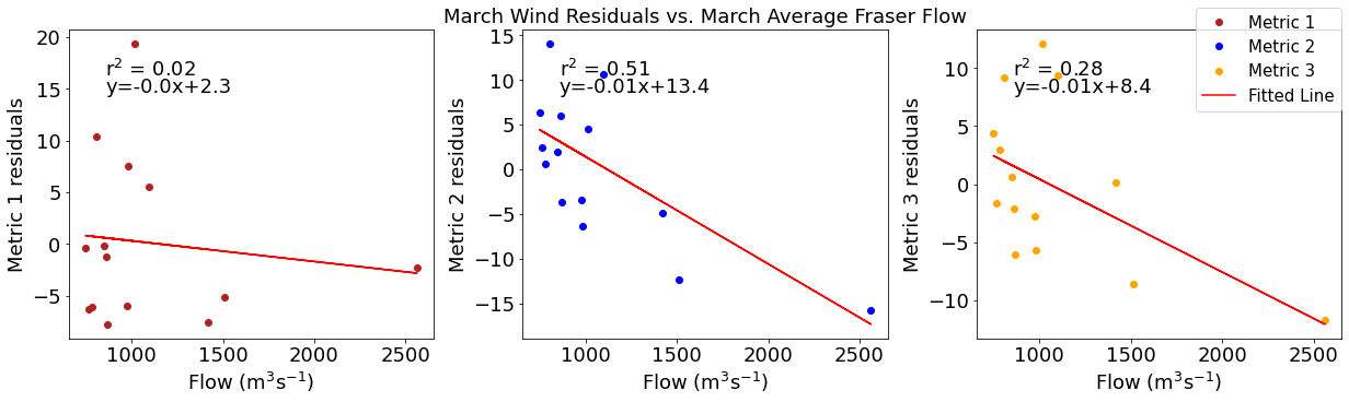
# ---------- Fraser ---------
fig4,ax4=plt.subplots(1,3,figsize=(17,5),constrained_layout=True)
ax4[0].plot(frasermar,windresid1,'o',color='firebrick',label='Metric 1')
ax4[0].set_xlabel('Flow (m$^3$s$^{-1}$)')
ax4[0].set_ylabel('Metric 1 residuals')
y,r2,m,b=bloomdrivers.reg_r2(frasermar,windresid1)
ax4[0].plot(frasermar, y, 'r')
ax4[0].text(0.1, 0.85, '$\mathregular{r^2}$ = %.2f'%r2, transform=ax4[0].transAxes)
ax4[0].text(0.1,0.78,f'y={round(m,2)}x+{round(b,1)}',horizontalalignment='left',verticalalignment='bottom',transform=ax4[0].transAxes)

ax4[1].plot(frasermar,windresid2,'o',color='b',label='Metric 2')
ax4[1].set_xlabel('Flow (m$^3$s$^{-1}$)')
ax4[1].set_ylabel('Metric 2 residuals')
ax4[1].set_title('March Wind Residuals vs. March Average Fraser Flow')
y,r2,m,b=bloomdrivers.reg_r2(frasermar,windresid2)
ax4[1].plot(frasermar, y, 'r')
ax4[1].text(0.1, 0.85, '$\mathregular{r^2}$ = %.2f'%r2, transform=ax4[1].transAxes)
ax4[1].text(0.1,0.78,f'y={round(m,2)}x+{round(b,1)}',horizontalalignment='left',verticalalignment='bottom',transform=ax4[1].transAxes)

ax4[2].plot(frasermar,windresid3,'o',color='orange',label='Metric 3')
ax4[2].set_xlabel('Flow (m$^3$s$^{-1}$)')
ax4[2].set_ylabel('Metric 3 residuals')
y,r2,m,b=bloomdrivers.reg_r2(frasermar,windresid3)
ax4[2].plot(frasermar, y, 'r', label='Fitted Line')
ax4[2].text(0.1, 0.85, '$\mathregular{r^2}$ = %.2f'%r2, transform=ax4[2].transAxes)
ax4[2].text(0.1,0.78,f'y={round(m,2)}x+{round(b,1)}',horizontalalignment='left',verticalalignment='bottom',transform=ax4[2].transAxes)
fig4.legend()
[25]:
<matplotlib.legend.Legend at 0x7f652ae9f280>
[26]:
# Wind residual calculations for each metric
windresid1b=list()
y,r2,m,b=bloomdrivers.reg_r2(windmar,yearday1)
#for ind,y in enumerate(yearday1):
#    x=windmar[ind]
#    windresid1b.append(y-(m*(x-np.mean(x))))
windresid1b=yearday1-m*(windmar-np.mean(windmar))

windresid2b=list()
y,r2,m,b=bloomdrivers.reg_r2(windmar,yearday2)
#for ind,y in enumerate(yearday2):
#    x=windmar[ind]
#    windresid2b.append(y-(m*(x-np.mean(x))))
windresid2b=yearday2-m*(windmar-np.mean(windmar))

windresid3b=list()
y,r2,m,b=bloomdrivers.reg_r2(windmar,yearday3)
#for ind,y in enumerate(yearday3):
#    x=windmar[ind]
#    windresid3b.append(y-(m*(x-np.mean(x))))
windresid3b=yearday3-m*(windmar-np.mean(windmar))
[27]:
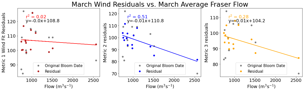
# ---------- Fraser ---------
fig4,ax4=plt.subplots(1,3,figsize=(17,5),constrained_layout=True)
ax4[0].plot(frasermar,yearday1,'o',color='gray',label='Original Bloom Date')
ax4[0].plot(frasermar,windresid1b,'o',color='firebrick',label='Residual')
ax4[0].set_xlabel('Flow (m$^3$s$^{-1}$)')
ax4[0].set_ylabel('Metric 1 Wind Fit Residuals')
y,r2,m,b=bloomdrivers.reg_r2(frasermar,windresid1b)
ax4[0].plot(frasermar, y, 'r')
ax4[0].text(0.1, 0.85, '$\mathregular{r^2}$ = %.2f'%r2, color='r',transform=ax4[0].transAxes)
ax4[0].text(0.1,0.78,f'y={round(m,2)}x+{round(b,1)}',horizontalalignment='left',verticalalignment='bottom',transform=ax4[0].transAxes)
ax4[0].legend(loc=8)

ax4[1].plot(frasermar,yearday2,'o',color='gray',label='Original Bloom Date')
ax4[1].plot(frasermar,windresid2b,'o',color='b',label='Residual')
ax4[1].set_xlabel('Flow (m$^3$s$^{-1}$)')
ax4[1].set_ylabel('Metric 2 residuals')
ax4[1].set_title('March Wind Residuals vs. March Average Fraser Flow',size=27)
y,r2,m,b=bloomdrivers.reg_r2(frasermar,windresid2b)
ax4[1].plot(frasermar, y, 'b')
ax4[1].text(0.1, 0.85, '$\mathregular{r^2}$ = %.2f'%r2,color='b', transform=ax4[1].transAxes)
ax4[1].text(0.1,0.78,f'y={round(m,2)}x+{round(b,1)}',horizontalalignment='left',verticalalignment='bottom',transform=ax4[1].transAxes)
ax4[1].legend(loc=8)

ax4[2].plot(frasermar,yearday3,'o',color='gray',label='Original Bloom Date')
ax4[2].plot(frasermar,windresid3b,'o',color='orange',label='Residual')
ax4[2].set_xlabel('Flow (m$^3$s$^{-1}$)')
ax4[2].set_ylabel('Metric 3 residuals')
y,r2,m,b=bloomdrivers.reg_r2(frasermar,windresid3b)
ax4[2].plot(frasermar, y, 'orange')
ax4[2].text(0.1, 0.85, '$\mathregular{r^2}$ = %.2f'%r2,color='orange', transform=ax4[2].transAxes)
ax4[2].text(0.1,0.78,f'y={round(m,2)}x+{round(b,1)}',horizontalalignment='left',verticalalignment='bottom',transform=ax4[2].transAxes)
#fig4.legend()
ax4[2].legend(loc=8)
[27]:
<matplotlib.legend.Legend at 0x7f652ad56f40>
[28]:
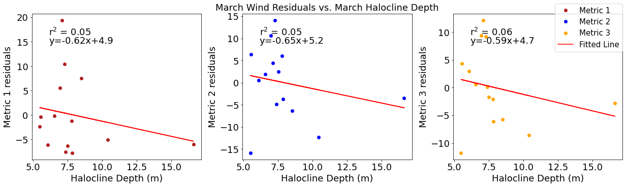
# ---------- Halocline ---------
fig4,ax4=plt.subplots(1,3,figsize=(17,5),constrained_layout=True)
ax4[0].plot(halomar,windresid1,'o',color='firebrick',label='Metric 1')
ax4[0].set_xlabel('Halocline Depth (m)')
ax4[0].set_ylabel('Metric 1 residuals')
y,r2,m,b=bloomdrivers.reg_r2(halomar,windresid1)
ax4[0].plot(halomar, y, 'r')
ax4[0].text(0.1, 0.85, '$\mathregular{r^2}$ = %.2f'%r2, transform=ax4[0].transAxes)
ax4[0].text(0.1,0.78,f'y={round(m,2)}x+{round(b,1)}',horizontalalignment='left',verticalalignment='bottom',transform=ax4[0].transAxes)

ax4[1].plot(halomar,windresid2,'o',color='b',label='Metric 2')
ax4[1].set_xlabel('Halocline Depth (m)')
ax4[1].set_ylabel('Metric 2 residuals')
ax4[1].set_title('March Wind Residuals vs. March Halocline Depth')
y,r2,m,b=bloomdrivers.reg_r2(halomar,windresid2)
ax4[1].plot(halomar, y, 'r')
ax4[1].text(0.1, 0.85, '$\mathregular{r^2}$ = %.2f'%r2, transform=ax4[1].transAxes)
ax4[1].text(0.1,0.78,f'y={round(m,2)}x+{round(b,1)}',horizontalalignment='left',verticalalignment='bottom',transform=ax4[1].transAxes)

ax4[2].plot(halomar,windresid3,'o',color='orange',label='Metric 3')
ax4[2].set_xlabel('Halocline Depth (m)')
ax4[2].set_ylabel('Metric 3 residuals')
y,r2,m,b=bloomdrivers.reg_r2(halomar,windresid3)
ax4[2].plot(halomar, y, 'r', label='Fitted Line')
ax4[2].text(0.1, 0.85, '$\mathregular{r^2}$ = %.2f'%r2, transform=ax4[2].transAxes)
ax4[2].text(0.1,0.78,f'y={round(m,2)}x+{round(b,1)}',horizontalalignment='left',verticalalignment='bottom',transform=ax4[2].transAxes)
fig4.legend()
[28]:
<matplotlib.legend.Legend at 0x7f652ac09df0>
Correlation plots of solar radiation residuals
[29]:
#  residual calculations for each metric
solarresid1=list()
y,r2,m,b=bloomdrivers.reg_r2(solarmar,yearday1)
for ind,y in enumerate(yearday1):
    x=solarmar[ind]
    solarresid1.append(y-(m*x+b))

solarresid2=list()
y,r2,m,b=bloomdrivers.reg_r2(solarmar,yearday2)
for ind,y in enumerate(yearday2):
    x=solarmar[ind]
    solarresid2.append(y-(m*x+b))

solarresid3=list()
y,r2,m,b=bloomdrivers.reg_r2(solarmar,yearday3)
for ind,y in enumerate(yearday3):
    x=solarmar[ind]
    solarresid3.append(y-(m*x+b))
[30]:
dfsolar=pd.DataFrame({'solar':solarmar,'solarresid1':solarresid1,'solarresid2':solarresid2,'solarresid3':solarresid3,'wind':windmar,
                  'temp':tempmar,'sal':salmar,'midno3':midno3mar,'fraser':frasermar,'deepno3':deepno3mar,'halocine':halomar})
[31]:
plt.subplots(figsize=(20,15))
cm1=cmocean.cm.curl
sns.heatmap(dfsolar.corr(), annot = True,cmap=cm1,vmin=-1,vmax=1)
[31]:
<AxesSubplot:>
[32]:
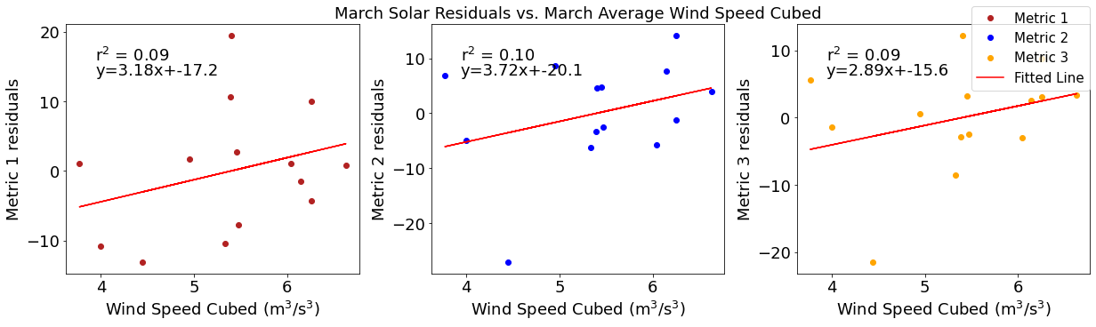
# ---------- wind ---------
fig4,ax4=plt.subplots(1,3,figsize=(17,5),constrained_layout=True)
ax4[0].plot(windmar,solarresid1,'o',color='firebrick',label='Metric 1')
ax4[0].set_xlabel('Wind Speed Cubed ($\mathregular{m^3}$/$\mathregular{s^3}$)')
ax4[0].set_ylabel('Metric 1 residuals')
y,r2,m,b=bloomdrivers.reg_r2(windmar,solarresid1)
ax4[0].plot(windmar, y, 'r')
ax4[0].text(0.1, 0.85, '$\mathregular{r^2}$ = %.2f'%r2, transform=ax4[0].transAxes)
ax4[0].text(0.1,0.78,f'y={round(m,2)}x+{round(b,1)}',horizontalalignment='left',verticalalignment='bottom',transform=ax4[0].transAxes)

ax4[1].plot(windmar,solarresid2,'o',color='b',label='Metric 2')
ax4[1].set_xlabel('Wind Speed Cubed ($\mathregular{m^3}$/$\mathregular{s^3}$)')
ax4[1].set_ylabel('Metric 2 residuals')
ax4[1].set_title('March Solar Residuals vs. March Average Wind Speed Cubed')
y,r2,m,b=bloomdrivers.reg_r2(windmar,solarresid2)
ax4[1].plot(windmar, y, 'r')
ax4[1].text(0.1, 0.85, '$\mathregular{r^2}$ = %.2f'%r2, transform=ax4[1].transAxes)
ax4[1].text(0.1,0.78,f'y={round(m,2)}x+{round(b,1)}',horizontalalignment='left',verticalalignment='bottom',transform=ax4[1].transAxes)

ax4[2].plot(windmar,solarresid3,'o',color='orange',label='Metric 3')
ax4[2].set_xlabel('Wind Speed Cubed ($\mathregular{m^3}$/$\mathregular{s^3}$)')
ax4[2].set_ylabel('Metric 3 residuals')
y,r2,m,b=bloomdrivers.reg_r2(windmar,solarresid3)
ax4[2].plot(windmar, y, 'r', label='Fitted Line')
ax4[2].text(0.1, 0.85, '$\mathregular{r^2}$ = %.2f'%r2, transform=ax4[2].transAxes)
ax4[2].text(0.1,0.78,f'y={round(m,2)}x+{round(b,1)}',horizontalalignment='left',verticalalignment='bottom',transform=ax4[2].transAxes)
fig4.legend()
[32]:
<matplotlib.legend.Legend at 0x7f652aa189d0>
[33]:
# ---------- Temperature ---------
fig4,ax4=plt.subplots(1,3,figsize=(17,5),constrained_layout=True)
ax4[0].plot(tempmar,solarresid1,'o',color='firebrick',label='Metric 1')
ax4[0].set_xlabel('Surface Temperature ($^\circ$C)')
ax4[0].set_ylabel('Metric 1 residuals')
y,r2,m,b=bloomdrivers.reg_r2(tempmar,solarresid1)
ax4[0].plot(tempmar, y, 'r')
ax4[0].text(0.1, 0.85, '$\mathregular{r^2}$ = %.2f'%r2, transform=ax4[0].transAxes)
ax4[0].text(0.1,0.78,f'y={round(m,2)}x+{round(b,1)}',horizontalalignment='left',verticalalignment='bottom',transform=ax4[0].transAxes)

ax4[1].plot(tempmar,solarresid2,'o',color='b',label='Metric 2')
ax4[1].set_xlabel('Surface Temperature ($^\circ$C)')
ax4[1].set_ylabel('Metric 2 residuals')
ax4[1].set_title('March Solar Residuals vs. March Average Surface Temperature')
y,r2,m,b=bloomdrivers.reg_r2(tempmar,solarresid2)
ax4[1].plot(tempmar, y, 'r')
ax4[1].text(0.1, 0.85, '$\mathregular{r^2}$ = %.2f'%r2, transform=ax4[1].transAxes)
ax4[1].text(0.1,0.78,f'y={round(m,2)}x+{round(b,1)}',horizontalalignment='left',verticalalignment='bottom',transform=ax4[1].transAxes)

ax4[2].plot(tempmar,solarresid3,'o',color='orange',label='Metric 3')
ax4[2].set_xlabel('Surface Temperature ($^\circ$C)')
ax4[2].set_ylabel('Metric 3 residuals')
y,r2,m,b=bloomdrivers.reg_r2(tempmar,solarresid3)
ax4[2].plot(tempmar, y, 'r', label='Fitted Line')
ax4[2].text(0.1, 0.85, '$\mathregular{r^2}$ = %.2f'%r2, transform=ax4[2].transAxes)
ax4[2].text(0.1,0.78,f'y={round(m,2)}x+{round(b,1)}',horizontalalignment='left',verticalalignment='bottom',transform=ax4[2].transAxes)
fig4.legend()
[33]:
<matplotlib.legend.Legend at 0x7f652a9344f0>
[34]:
# ---------- Mid NO3 ---------
fig4,ax4=plt.subplots(1,3,figsize=(17,5),constrained_layout=True)
ax4[0].plot(midno3mar,solarresid1,'o',color='firebrick',label='Metric 1')
ax4[0].set_xlabel('Concentration ($\mu$M N)')
ax4[0].set_ylabel('Metric 1 residuals')
y,r2,m,b=bloomdrivers.reg_r2(midno3mar,solarresid1)
ax4[0].plot(midno3mar, y, 'r')
ax4[0].text(0.1, 0.85, '$\mathregular{r^2}$ = %.2f'%r2, transform=ax4[0].transAxes)
ax4[0].text(0.1,0.78,f'y={round(m,2)}x+{round(b,1)}',horizontalalignment='left',verticalalignment='bottom',transform=ax4[0].transAxes)
ax4[1].plot(midno3mar,solarresid2,'o',color='b',label='Metric 2')
ax4[1].set_xlabel('Concentration ($\mu$M N)')
ax4[1].set_ylabel('Metric 2 residuals')
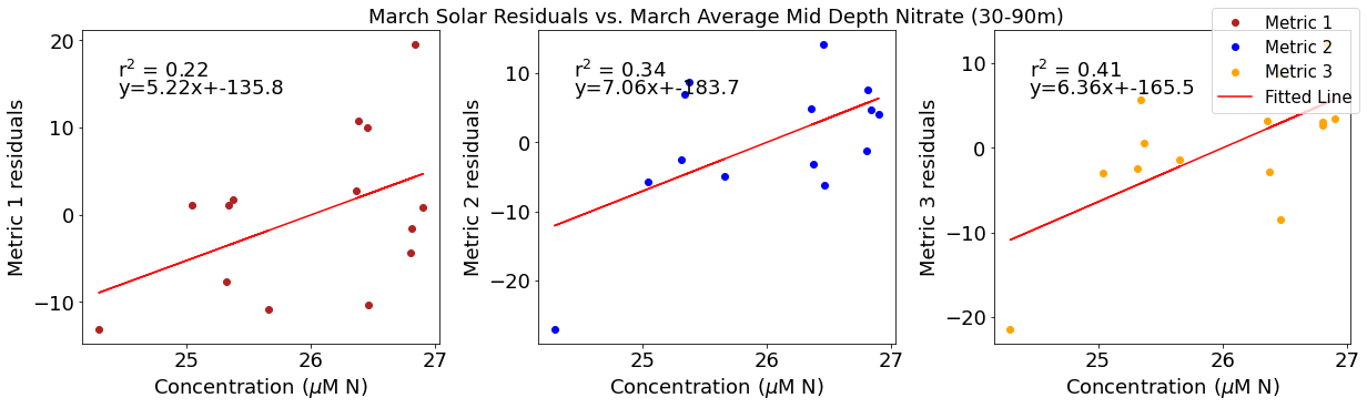
ax4[1].set_title('March Solar Residuals vs. March Average Mid Depth Nitrate (30-90m)')
y,r2,m,b=bloomdrivers.reg_r2(midno3mar,solarresid2)
ax4[1].plot(midno3mar, y, 'r')
ax4[1].text(0.1, 0.85, '$\mathregular{r^2}$ = %.2f'%r2, transform=ax4[1].transAxes)
ax4[1].text(0.1,0.78,f'y={round(m,2)}x+{round(b,1)}',horizontalalignment='left',verticalalignment='bottom',transform=ax4[1].transAxes)
ax4[2].plot(midno3mar,solarresid3,'o',color='orange',label='Metric 3')
ax4[2].set_xlabel('Concentration ($\mu$M N)')
ax4[2].set_ylabel('Metric 3 residuals')
y,r2,m,b=bloomdrivers.reg_r2(midno3mar,solarresid3)
ax4[2].plot(midno3mar, y, 'r', label='Fitted Line')
ax4[2].text(0.1, 0.85, '$\mathregular{r^2}$ = %.2f'%r2, transform=ax4[2].transAxes)
ax4[2].text(0.1,0.78,f'y={round(m,2)}x+{round(b,1)}',horizontalalignment='left',verticalalignment='bottom',transform=ax4[2].transAxes)
fig4.legend()
[34]:
<matplotlib.legend.Legend at 0x7f652a7c2bb0>
[35]:
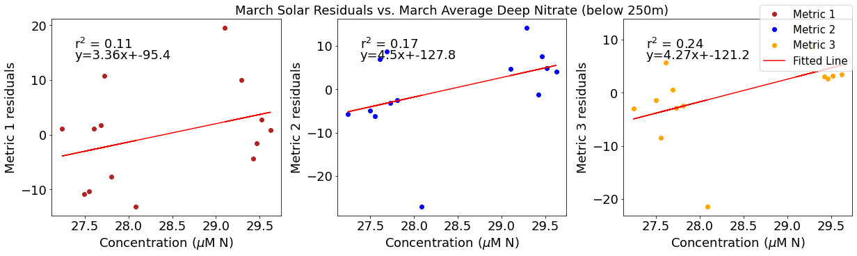
# ---------- Deep NO3 ---------
fig4,ax4=plt.subplots(1,3,figsize=(17,5),constrained_layout=True)
ax4[0].plot(deepno3mar,solarresid1,'o',color='firebrick',label='Metric 1')
ax4[0].set_xlabel('Concentration ($\mu$M N)')
ax4[0].set_ylabel('Metric 1 residuals')
y,r2,m,b=bloomdrivers.reg_r2(deepno3mar,solarresid1)
ax4[0].plot(deepno3mar, y, 'r')
ax4[0].text(0.1, 0.85, '$\mathregular{r^2}$ = %.2f'%r2, transform=ax4[0].transAxes)
ax4[0].text(0.1,0.78,f'y={round(m,2)}x+{round(b,1)}',horizontalalignment='left',verticalalignment='bottom',transform=ax4[0].transAxes)

ax4[1].plot(deepno3mar,solarresid2,'o',color='b',label='Metric 2')
ax4[1].set_xlabel('Concentration ($\mu$M N)')
ax4[1].set_ylabel('Metric 2 residuals')
ax4[1].set_title('March Solar Residuals vs. March Average Deep Nitrate (below 250m)')
y,r2,m,b=bloomdrivers.reg_r2(deepno3mar,solarresid2)
ax4[1].plot(deepno3mar, y, 'r')
ax4[1].text(0.1, 0.85, '$\mathregular{r^2}$ = %.2f'%r2, transform=ax4[1].transAxes)
ax4[1].text(0.1,0.78,f'y={round(m,2)}x+{round(b,1)}',horizontalalignment='left',verticalalignment='bottom',transform=ax4[1].transAxes)

ax4[2].plot(deepno3mar,solarresid3,'o',color='orange',label='Metric 3')
ax4[2].set_xlabel('Concentration ($\mu$M N)')
ax4[2].set_ylabel('Metric 3 residuals')
y,r2,m,b=bloomdrivers.reg_r2(deepno3mar,solarresid3)
ax4[2].plot(deepno3mar, y, 'r', label='Fitted Line')
ax4[2].text(0.1, 0.85, '$\mathregular{r^2}$ = %.2f'%r2, transform=ax4[2].transAxes)
ax4[2].text(0.1,0.78,f'y={round(m,2)}x+{round(b,1)}',horizontalalignment='left',verticalalignment='bottom',transform=ax4[2].transAxes)
fig4.legend()
[35]:
<matplotlib.legend.Legend at 0x7f652a6dc3a0>
[36]:
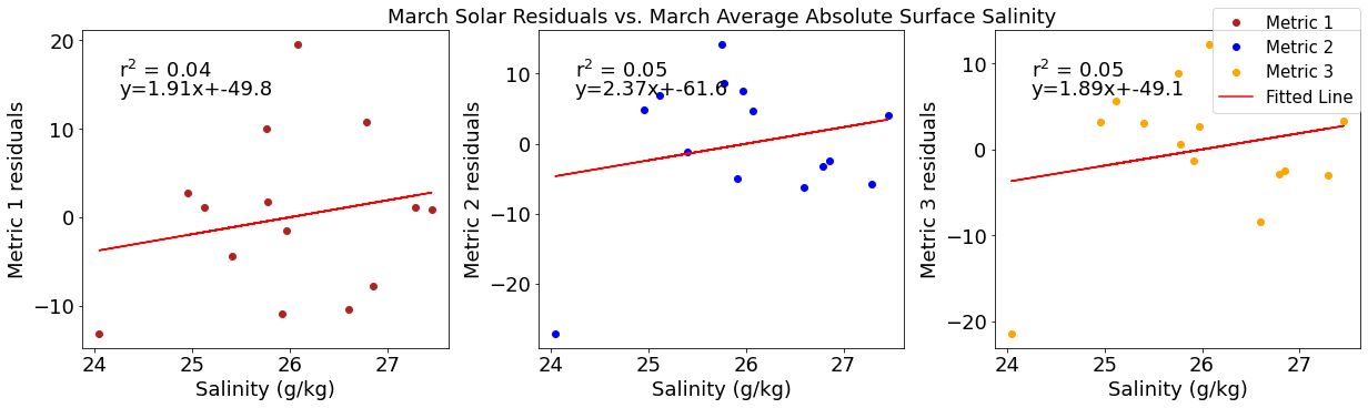
# ---------- Salinity ---------
fig4,ax4=plt.subplots(1,3,figsize=(17,5),constrained_layout=True)
ax4[0].plot(salmar,solarresid1,'o',color='firebrick',label='Metric 1')
ax4[0].set_xlabel('Salinity (g/kg)')
ax4[0].set_ylabel('Metric 1 residuals')
y,r2,m,b=bloomdrivers.reg_r2(salmar,solarresid1)
ax4[0].plot(salmar, y, 'r')
ax4[0].text(0.1, 0.85, '$\mathregular{r^2}$ = %.2f'%r2, transform=ax4[0].transAxes)
ax4[0].text(0.1,0.78,f'y={round(m,2)}x+{round(b,1)}',horizontalalignment='left',verticalalignment='bottom',transform=ax4[0].transAxes)

ax4[1].plot(salmar,solarresid2,'o',color='b',label='Metric 2')
ax4[1].set_xlabel('Salinity (g/kg)')
ax4[1].set_ylabel('Metric 2 residuals')
ax4[1].set_title('March Solar Residuals vs. March Average Absolute Surface Salinity')
y,r2,m,b=bloomdrivers.reg_r2(salmar,solarresid2)
ax4[1].plot(salmar, y, 'r')
ax4[1].text(0.1, 0.85, '$\mathregular{r^2}$ = %.2f'%r2, transform=ax4[1].transAxes)
ax4[1].text(0.1,0.78,f'y={round(m,2)}x+{round(b,1)}',horizontalalignment='left',verticalalignment='bottom',transform=ax4[1].transAxes)

ax4[2].plot(salmar,solarresid3,'o',color='orange',label='Metric 3')
ax4[2].set_xlabel('Salinity (g/kg)')
ax4[2].set_ylabel('Metric 3 residuals')
y,r2,m,b=bloomdrivers.reg_r2(salmar,solarresid3)
ax4[2].plot(salmar, y, 'r', label='Fitted Line')
ax4[2].text(0.1, 0.85, '$\mathregular{r^2}$ = %.2f'%r2, transform=ax4[2].transAxes)
ax4[2].text(0.1,0.78,f'y={round(m,2)}x+{round(b,1)}',horizontalalignment='left',verticalalignment='bottom',transform=ax4[2].transAxes)
fig4.legend()
[36]:
<matplotlib.legend.Legend at 0x7f652a5fa7c0>
[37]:
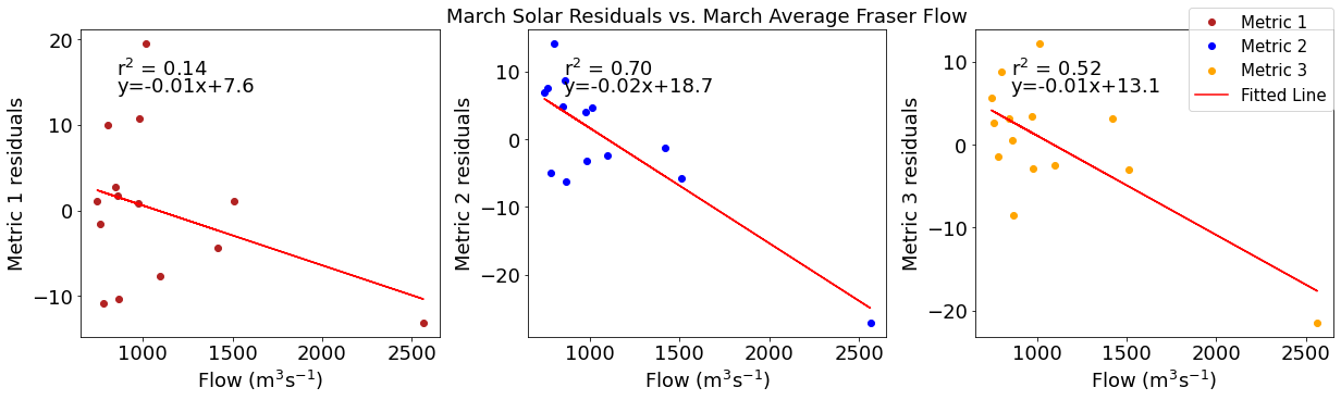
# ---------- Fraser ---------
fig4,ax4=plt.subplots(1,3,figsize=(17,5),constrained_layout=True)
ax4[0].plot(frasermar,solarresid1,'o',color='firebrick',label='Metric 1')
ax4[0].set_xlabel('Flow (m$^3$s$^{-1}$)')
ax4[0].set_ylabel('Metric 1 residuals')
y,r2,m,b=bloomdrivers.reg_r2(frasermar,solarresid1)
ax4[0].plot(frasermar, y, 'r')
ax4[0].text(0.1, 0.85, '$\mathregular{r^2}$ = %.2f'%r2, transform=ax4[0].transAxes)
ax4[0].text(0.1,0.78,f'y={round(m,2)}x+{round(b,1)}',horizontalalignment='left',verticalalignment='bottom',transform=ax4[0].transAxes)

ax4[1].plot(frasermar,solarresid2,'o',color='b',label='Metric 2')
ax4[1].set_xlabel('Flow (m$^3$s$^{-1}$)')
ax4[1].set_ylabel('Metric 2 residuals')
ax4[1].set_title('March Solar Residuals vs. March Average Fraser Flow')
y,r2,m,b=bloomdrivers.reg_r2(frasermar,solarresid2)
ax4[1].plot(frasermar, y, 'r')
ax4[1].text(0.1, 0.85, '$\mathregular{r^2}$ = %.2f'%r2, transform=ax4[1].transAxes)
ax4[1].text(0.1,0.78,f'y={round(m,2)}x+{round(b,1)}',horizontalalignment='left',verticalalignment='bottom',transform=ax4[1].transAxes)

ax4[2].plot(frasermar,solarresid3,'o',color='orange',label='Metric 3')
ax4[2].set_xlabel('Flow (m$^3$s$^{-1}$)')
ax4[2].set_ylabel('Metric 3 residuals')
y,r2,m,b=bloomdrivers.reg_r2(frasermar,solarresid3)
ax4[2].plot(frasermar, y, 'r', label='Fitted Line')
ax4[2].text(0.1, 0.85, '$\mathregular{r^2}$ = %.2f'%r2, transform=ax4[2].transAxes)
ax4[2].text(0.1,0.78,f'y={round(m,2)}x+{round(b,1)}',horizontalalignment='left',verticalalignment='bottom',transform=ax4[2].transAxes)
fig4.legend()
[37]:
<matplotlib.legend.Legend at 0x7f652a4fe850>
[38]:
# ---------- Halocline ---------
fig4,ax4=plt.subplots(1,3,figsize=(17,5),constrained_layout=True)
ax4[0].plot(halomar,solarresid1,'o',color='firebrick',label='Metric 1')
ax4[0].set_xlabel('Halocline Depth (m)')
ax4[0].set_ylabel('Metric 1 residuals')
y,r2,m,b=bloomdrivers.reg_r2(halomar,solarresid1)
ax4[0].plot(halomar, y, 'r')
ax4[0].text(0.1, 0.85, '$\mathregular{r^2}$ = %.2f'%r2, transform=ax4[0].transAxes)
ax4[0].text(0.1,0.78,f'y={round(m,2)}x+{round(b,1)}',horizontalalignment='left',verticalalignment='bottom',transform=ax4[0].transAxes)
ax4[1].plot(halomar,solarresid2,'o',color='b',label='Metric 2')
ax4[1].set_xlabel('Halocline Depth (m)')
ax4[1].set_ylabel('Metric 2 residuals')
ax4[1].set_title('March Solar Residuals vs. March Halocline Depth')
y,r2,m,b=bloomdrivers.reg_r2(halomar,solarresid2)
ax4[1].plot(halomar, y, 'r')
ax4[1].text(0.1, 0.85, '$\mathregular{r^2}$ = %.2f'%r2, transform=ax4[1].transAxes)
ax4[1].text(0.1,0.78,f'y={round(m,2)}x+{round(b,1)}',horizontalalignment='left',verticalalignment='bottom',transform=ax4[1].transAxes)
ax4[2].plot(halomar,solarresid3,'o',color='orange',label='Metric 3')
ax4[2].set_xlabel('Halocline Depth (m)')
ax4[2].set_ylabel('Metric 3 residuals')
y,r2,m,b=bloomdrivers.reg_r2(halomar,solarresid3)
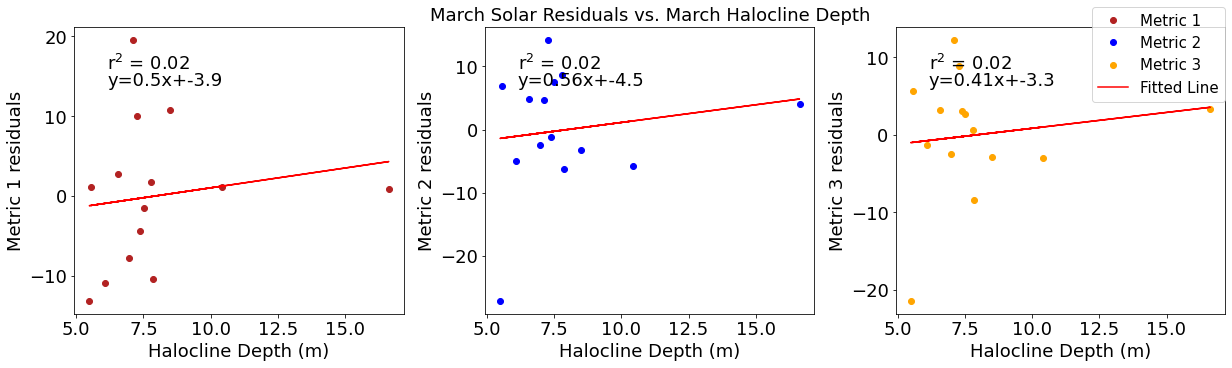
ax4[2].plot(halomar, y, 'r', label='Fitted Line')
ax4[2].text(0.1, 0.85, '$\mathregular{r^2}$ = %.2f'%r2, transform=ax4[2].transAxes)
ax4[2].text(0.1,0.78,f'y={round(m,2)}x+{round(b,1)}',horizontalalignment='left',verticalalignment='bottom',transform=ax4[2].transAxes)
fig4.legend()
[38]:
<matplotlib.legend.Legend at 0x7f652a3818b0>
Correlation plots of temperature residuals
[39]:
#  residual calculations for each metric
tempresid1=list()
y,r2,m,b=bloomdrivers.reg_r2(tempmar,yearday1)
for ind,y in enumerate(yearday1):
    x=tempmar[ind]
    tempresid1.append(y-(m*x+b))

tempresid2=list()
y,r2,m,b=bloomdrivers.reg_r2(tempmar,yearday2)
for ind,y in enumerate(yearday2):
    x=tempmar[ind]
    tempresid2.append(y-(m*x+b))

tempresid3=list()
y,r2,m,b=bloomdrivers.reg_r2(tempmar,yearday3)
for ind,y in enumerate(yearday3):
    x=tempmar[ind]
    tempresid3.append(y-(m*x+b))
[40]:
dftemp=pd.DataFrame({'temp':tempmar,'tempresid1':tempresid1,'tempresid2':tempresid2,'tempresid3':tempresid3,'wind':windmar,'solar':solarmar,
                  'sal':salmar,'midno3':midno3mar,'fraser':frasermar,'deepno3':deepno3mar,'halocine':halomar})
[41]:
plt.subplots(figsize=(20,15))
cm1=cmocean.cm.curl
sns.heatmap(dftemp.corr(), annot = True,cmap=cm1,vmin=-1,vmax=1)
[41]:
<AxesSubplot:>
[42]:
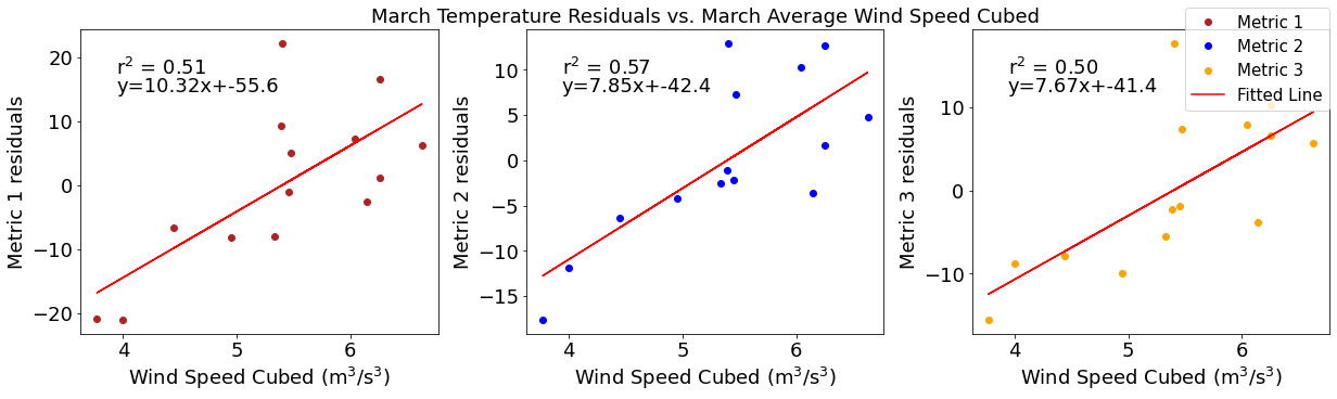
# ---------- wind ---------
fig4,ax4=plt.subplots(1,3,figsize=(17,5),constrained_layout=True)
ax4[0].plot(windmar,tempresid1,'o',color='firebrick',label='Metric 1')
ax4[0].set_xlabel('Wind Speed Cubed ($\mathregular{m^3}$/$\mathregular{s^3}$)')
ax4[0].set_ylabel('Metric 1 residuals')
y,r2,m,b=bloomdrivers.reg_r2(windmar,tempresid1)
ax4[0].plot(windmar, y, 'r')
ax4[0].text(0.1, 0.85, '$\mathregular{r^2}$ = %.2f'%r2, transform=ax4[0].transAxes)
ax4[0].text(0.1,0.78,f'y={round(m,2)}x+{round(b,1)}',horizontalalignment='left',verticalalignment='bottom',transform=ax4[0].transAxes)

ax4[1].plot(windmar,tempresid2,'o',color='b',label='Metric 2')
ax4[1].set_xlabel('Wind Speed Cubed ($\mathregular{m^3}$/$\mathregular{s^3}$)')
ax4[1].set_ylabel('Metric 2 residuals')
ax4[1].set_title('March Temperature Residuals vs. March Average Wind Speed Cubed')
y,r2,m,b=bloomdrivers.reg_r2(windmar,tempresid2)
ax4[1].plot(windmar, y, 'r')
ax4[1].text(0.1, 0.85, '$\mathregular{r^2}$ = %.2f'%r2, transform=ax4[1].transAxes)
ax4[1].text(0.1,0.78,f'y={round(m,2)}x+{round(b,1)}',horizontalalignment='left',verticalalignment='bottom',transform=ax4[1].transAxes)

ax4[2].plot(windmar,tempresid3,'o',color='orange',label='Metric 3')
ax4[2].set_xlabel('Wind Speed Cubed ($\mathregular{m^3}$/$\mathregular{s^3}$)')
ax4[2].set_ylabel('Metric 3 residuals')
y,r2,m,b=bloomdrivers.reg_r2(windmar,tempresid3)
ax4[2].plot(windmar, y, 'r', label='Fitted Line')
ax4[2].text(0.1, 0.85, '$\mathregular{r^2}$ = %.2f'%r2, transform=ax4[2].transAxes)
ax4[2].text(0.1,0.78,f'y={round(m,2)}x+{round(b,1)}',horizontalalignment='left',verticalalignment='bottom',transform=ax4[2].transAxes)
fig4.legend()
[42]:
<matplotlib.legend.Legend at 0x7f652a9ed370>
[43]:
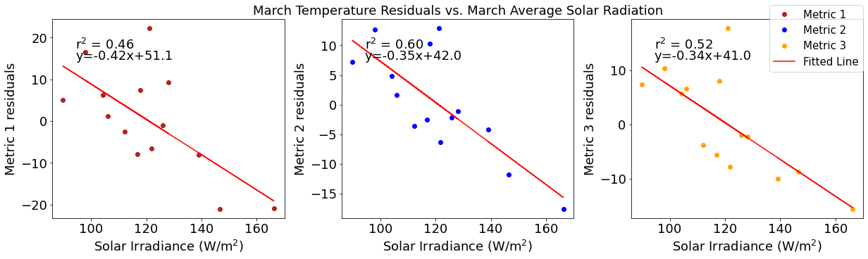
# ---------- Solar ---------
fig4,ax4=plt.subplots(1,3,figsize=(17,5),constrained_layout=True)
ax4[0].plot(solarmar,tempresid1,'o',color='firebrick',label='Metric 1')
ax4[0].set_xlabel('Solar Irradiance (W/$\mathregular{m^2}$)')
ax4[0].set_ylabel('Metric 1 residuals')
y,r2,m,b=bloomdrivers.reg_r2(solarmar,tempresid1)
ax4[0].plot(solarmar, y, 'r')
ax4[0].text(0.1, 0.85, '$\mathregular{r^2}$ = %.2f'%r2, transform=ax4[0].transAxes)
ax4[0].text(0.1,0.78,f'y={round(m,2)}x+{round(b,1)}',horizontalalignment='left',verticalalignment='bottom',transform=ax4[0].transAxes)

ax4[1].plot(solarmar,tempresid2,'o',color='b',label='Metric 2')
ax4[1].set_xlabel('Solar Irradiance (W/$\mathregular{m^2}$)')
ax4[1].set_ylabel('Metric 2 residuals')
ax4[1].set_title('March Temperature Residuals vs. March Average Solar Radiation')
y,r2,m,b=bloomdrivers.reg_r2(solarmar,tempresid2)
ax4[1].plot(solarmar, y, 'r')
ax4[1].text(0.1, 0.85, '$\mathregular{r^2}$ = %.2f'%r2, transform=ax4[1].transAxes)
ax4[1].text(0.1,0.78,f'y={round(m,2)}x+{round(b,1)}',horizontalalignment='left',verticalalignment='bottom',transform=ax4[1].transAxes)

ax4[2].plot(solarmar,tempresid3,'o',color='orange',label='Metric 3')
ax4[2].set_xlabel('Solar Irradiance (W/$\mathregular{m^2}$)')
ax4[2].set_ylabel('Metric 3 residuals')
y,r2,m,b=bloomdrivers.reg_r2(solarmar,tempresid3)
ax4[2].plot(solarmar, y, 'r', label='Fitted Line')
ax4[2].text(0.1, 0.85, '$\mathregular{r^2}$ = %.2f'%r2, transform=ax4[2].transAxes)
ax4[2].text(0.1,0.78,f'y={round(m,2)}x+{round(b,1)}',horizontalalignment='left',verticalalignment='bottom',transform=ax4[2].transAxes)
fig4.legend()
[43]:
<matplotlib.legend.Legend at 0x7f652a0a8f10>
[44]:
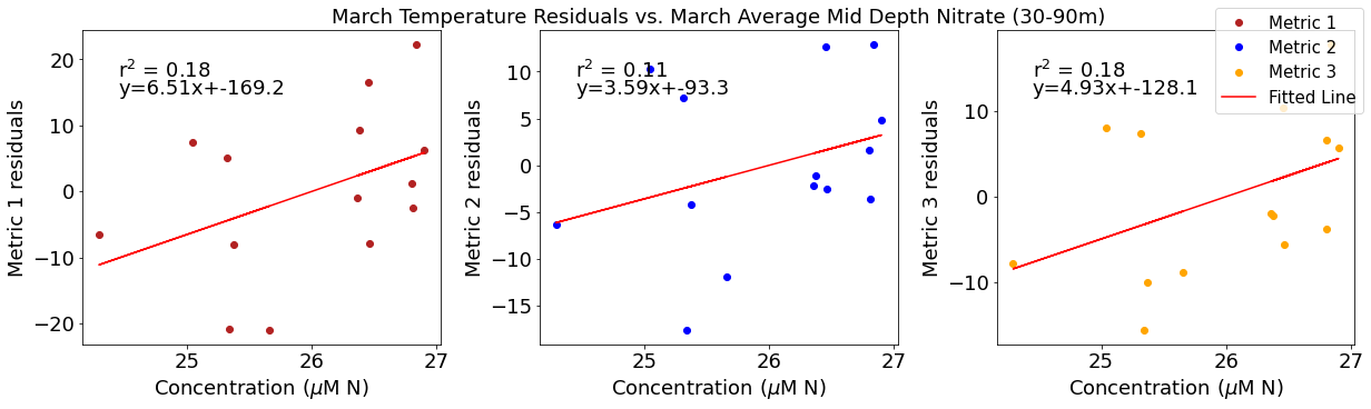
# ---------- Mid NO3 ---------
fig4,ax4=plt.subplots(1,3,figsize=(17,5),constrained_layout=True)
ax4[0].plot(midno3mar,tempresid1,'o',color='firebrick',label='Metric 1')
ax4[0].set_xlabel('Concentration ($\mu$M N)')
ax4[0].set_ylabel('Metric 1 residuals')
y,r2,m,b=bloomdrivers.reg_r2(midno3mar,tempresid1)
ax4[0].plot(midno3mar, y, 'r')
ax4[0].text(0.1, 0.85, '$\mathregular{r^2}$ = %.2f'%r2, transform=ax4[0].transAxes)
ax4[0].text(0.1,0.78,f'y={round(m,2)}x+{round(b,1)}',horizontalalignment='left',verticalalignment='bottom',transform=ax4[0].transAxes)

ax4[1].plot(midno3mar,tempresid2,'o',color='b',label='Metric 2')
ax4[1].set_xlabel('Concentration ($\mu$M N)')
ax4[1].set_ylabel('Metric 2 residuals')
ax4[1].set_title('March Temperature Residuals vs. March Average Mid Depth Nitrate (30-90m)')
y,r2,m,b=bloomdrivers.reg_r2(midno3mar,tempresid2)
ax4[1].plot(midno3mar, y, 'r')
ax4[1].text(0.1, 0.85, '$\mathregular{r^2}$ = %.2f'%r2, transform=ax4[1].transAxes)
ax4[1].text(0.1,0.78,f'y={round(m,2)}x+{round(b,1)}',horizontalalignment='left',verticalalignment='bottom',transform=ax4[1].transAxes)

ax4[2].plot(midno3mar,tempresid3,'o',color='orange',label='Metric 3')
ax4[2].set_xlabel('Concentration ($\mu$M N)')
ax4[2].set_ylabel('Metric 3 residuals')
y,r2,m,b=bloomdrivers.reg_r2(midno3mar,tempresid3)
ax4[2].plot(midno3mar, y, 'r', label='Fitted Line')
ax4[2].text(0.1, 0.85, '$\mathregular{r^2}$ = %.2f'%r2, transform=ax4[2].transAxes)
ax4[2].text(0.1,0.78,f'y={round(m,2)}x+{round(b,1)}',horizontalalignment='left',verticalalignment='bottom',transform=ax4[2].transAxes)
fig4.legend()
[44]:
<matplotlib.legend.Legend at 0x7f6529f49460>
[45]:
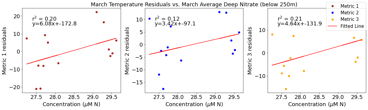
# ---------- Deep NO3 ---------
fig4,ax4=plt.subplots(1,3,figsize=(17,5),constrained_layout=True)
ax4[0].plot(deepno3mar,tempresid1,'o',color='firebrick',label='Metric 1')
ax4[0].set_xlabel('Concentration ($\mu$M N)')
ax4[0].set_ylabel('Metric 1 residuals')
y,r2,m,b=bloomdrivers.reg_r2(deepno3mar,tempresid1)
ax4[0].plot(deepno3mar, y, 'r')
ax4[0].text(0.1, 0.85, '$\mathregular{r^2}$ = %.2f'%r2, transform=ax4[0].transAxes)
ax4[0].text(0.1,0.78,f'y={round(m,2)}x+{round(b,1)}',horizontalalignment='left',verticalalignment='bottom',transform=ax4[0].transAxes)

ax4[1].plot(deepno3mar,tempresid2,'o',color='b',label='Metric 2')
ax4[1].set_xlabel('Concentration ($\mu$M N)')
ax4[1].set_ylabel('Metric 2 residuals')
ax4[1].set_title('March Temperature Residuals vs. March Average Deep Nitrate (below 250m)')
y,r2,m,b=bloomdrivers.reg_r2(deepno3mar,tempresid2)
ax4[1].plot(deepno3mar, y, 'r')
ax4[1].text(0.1, 0.85, '$\mathregular{r^2}$ = %.2f'%r2, transform=ax4[1].transAxes)
ax4[1].text(0.1,0.78,f'y={round(m,2)}x+{round(b,1)}',horizontalalignment='left',verticalalignment='bottom',transform=ax4[1].transAxes)

ax4[2].plot(deepno3mar,tempresid3,'o',color='orange',label='Metric 3')
ax4[2].set_xlabel('Concentration ($\mu$M N)')
ax4[2].set_ylabel('Metric 3 residuals')
y,r2,m,b=bloomdrivers.reg_r2(deepno3mar,tempresid3)
ax4[2].plot(deepno3mar, y, 'r', label='Fitted Line')
ax4[2].text(0.1, 0.85, '$\mathregular{r^2}$ = %.2f'%r2, transform=ax4[2].transAxes)
ax4[2].text(0.1,0.78,f'y={round(m,2)}x+{round(b,1)}',horizontalalignment='left',verticalalignment='bottom',transform=ax4[2].transAxes)
fig4.legend()
[45]:
<matplotlib.legend.Legend at 0x7f6529e61dc0>
[46]:
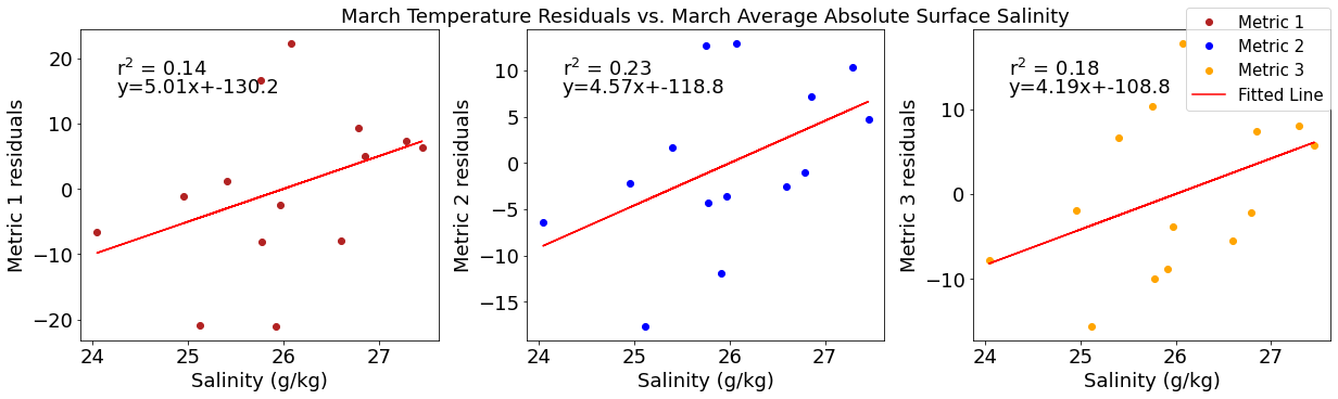
# ---------- Salinity ---------
fig4,ax4=plt.subplots(1,3,figsize=(17,5),constrained_layout=True)
ax4[0].plot(salmar,tempresid1,'o',color='firebrick',label='Metric 1')
ax4[0].set_xlabel('Salinity (g/kg)')
ax4[0].set_ylabel('Metric 1 residuals')
y,r2,m,b=bloomdrivers.reg_r2(salmar,tempresid1)
ax4[0].plot(salmar, y, 'r')
ax4[0].text(0.1, 0.85, '$\mathregular{r^2}$ = %.2f'%r2, transform=ax4[0].transAxes)
ax4[0].text(0.1,0.78,f'y={round(m,2)}x+{round(b,1)}',horizontalalignment='left',verticalalignment='bottom',transform=ax4[0].transAxes)

ax4[1].plot(salmar,tempresid2,'o',color='b',label='Metric 2')
ax4[1].set_xlabel('Salinity (g/kg)')
ax4[1].set_ylabel('Metric 2 residuals')
ax4[1].set_title('March Temperature Residuals vs. March Average Absolute Surface Salinity')
y,r2,m,b=bloomdrivers.reg_r2(salmar,tempresid2)
ax4[1].plot(salmar, y, 'r')
ax4[1].text(0.1, 0.85, '$\mathregular{r^2}$ = %.2f'%r2, transform=ax4[1].transAxes)
ax4[1].text(0.1,0.78,f'y={round(m,2)}x+{round(b,1)}',horizontalalignment='left',verticalalignment='bottom',transform=ax4[1].transAxes)

ax4[2].plot(salmar,tempresid3,'o',color='orange',label='Metric 3')
ax4[2].set_xlabel('Salinity (g/kg)')
ax4[2].set_ylabel('Metric 3 residuals')
y,r2,m,b=bloomdrivers.reg_r2(salmar,tempresid3)
ax4[2].plot(salmar, y, 'r', label='Fitted Line')
ax4[2].text(0.1, 0.85, '$\mathregular{r^2}$ = %.2f'%r2, transform=ax4[2].transAxes)
ax4[2].text(0.1,0.78,f'y={round(m,2)}x+{round(b,1)}',horizontalalignment='left',verticalalignment='bottom',transform=ax4[2].transAxes)
fig4.legend()
[46]:
<matplotlib.legend.Legend at 0x7f6529d04d60>
[47]:
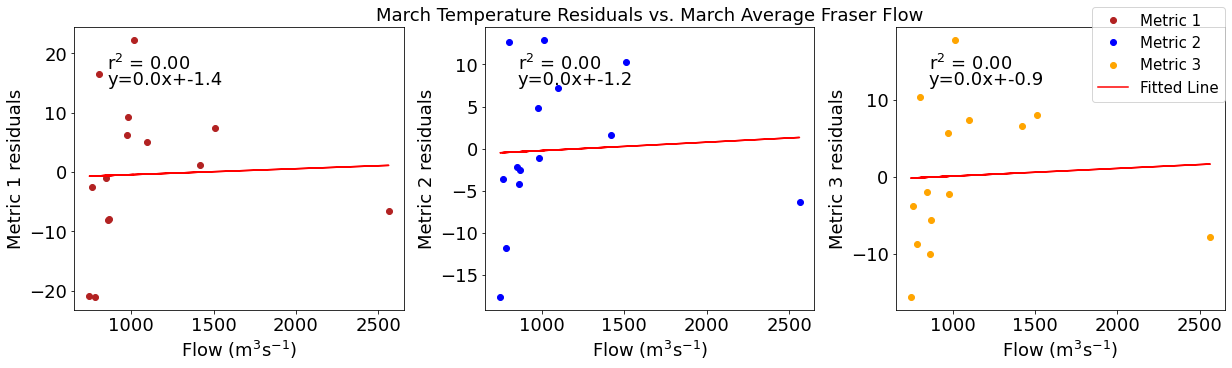
# ---------- Fraser ---------
fig4,ax4=plt.subplots(1,3,figsize=(17,5),constrained_layout=True)
ax4[0].plot(frasermar,tempresid1,'o',color='firebrick',label='Metric 1')
ax4[0].set_xlabel('Flow (m$^3$s$^{-1}$)')
ax4[0].set_ylabel('Metric 1 residuals')
y,r2,m,b=bloomdrivers.reg_r2(frasermar,tempresid1)
ax4[0].plot(frasermar, y, 'r')
ax4[0].text(0.1, 0.85, '$\mathregular{r^2}$ = %.2f'%r2, transform=ax4[0].transAxes)
ax4[0].text(0.1,0.78,f'y={round(m,2)}x+{round(b,1)}',horizontalalignment='left',verticalalignment='bottom',transform=ax4[0].transAxes)

ax4[1].plot(frasermar,tempresid2,'o',color='b',label='Metric 2')
ax4[1].set_xlabel('Flow (m$^3$s$^{-1}$)')
ax4[1].set_ylabel('Metric 2 residuals')
ax4[1].set_title('March Temperature Residuals vs. March Average Fraser Flow')
y,r2,m,b=bloomdrivers.reg_r2(frasermar,tempresid2)
ax4[1].plot(frasermar, y, 'r')
ax4[1].text(0.1, 0.85, '$\mathregular{r^2}$ = %.2f'%r2, transform=ax4[1].transAxes)
ax4[1].text(0.1,0.78,f'y={round(m,2)}x+{round(b,1)}',horizontalalignment='left',verticalalignment='bottom',transform=ax4[1].transAxes)

ax4[2].plot(frasermar,tempresid3,'o',color='orange',label='Metric 3')
ax4[2].set_xlabel('Flow (m$^3$s$^{-1}$)')
ax4[2].set_ylabel('Metric 3 residuals')
y,r2,m,b=bloomdrivers.reg_r2(frasermar,tempresid3)
ax4[2].plot(frasermar, y, 'r', label='Fitted Line')
ax4[2].text(0.1, 0.85, '$\mathregular{r^2}$ = %.2f'%r2, transform=ax4[2].transAxes)
ax4[2].text(0.1,0.78,f'y={round(m,2)}x+{round(b,1)}',horizontalalignment='left',verticalalignment='bottom',transform=ax4[2].transAxes)
fig4.legend()
[47]:
<matplotlib.legend.Legend at 0x7f6529c28310>
[48]:
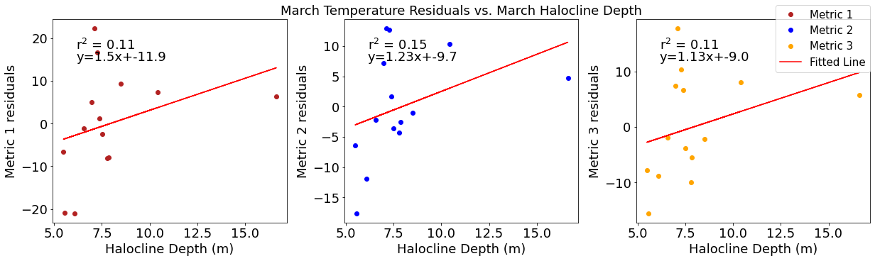
# ---------- Halocline ---------
fig4,ax4=plt.subplots(1,3,figsize=(17,5),constrained_layout=True)
ax4[0].plot(halomar,tempresid1,'o',color='firebrick',label='Metric 1')
ax4[0].set_xlabel('Halocline Depth (m)')
ax4[0].set_ylabel('Metric 1 residuals')
y,r2,m,b=bloomdrivers.reg_r2(halomar,tempresid1)
ax4[0].plot(halomar, y, 'r')
ax4[0].text(0.1, 0.85, '$\mathregular{r^2}$ = %.2f'%r2, transform=ax4[0].transAxes)
ax4[0].text(0.1,0.78,f'y={round(m,2)}x+{round(b,1)}',horizontalalignment='left',verticalalignment='bottom',transform=ax4[0].transAxes)

ax4[1].plot(halomar,tempresid2,'o',color='b',label='Metric 2')
ax4[1].set_xlabel('Halocline Depth (m)')
ax4[1].set_ylabel('Metric 2 residuals')
ax4[1].set_title('March Temperature Residuals vs. March Halocline Depth')
y,r2,m,b=bloomdrivers.reg_r2(halomar,tempresid2)
ax4[1].plot(halomar, y, 'r')
ax4[1].text(0.1, 0.85, '$\mathregular{r^2}$ = %.2f'%r2, transform=ax4[1].transAxes)
ax4[1].text(0.1,0.78,f'y={round(m,2)}x+{round(b,1)}',horizontalalignment='left',verticalalignment='bottom',transform=ax4[1].transAxes)

ax4[2].plot(halomar,tempresid3,'o',color='orange',label='Metric 3')
ax4[2].set_xlabel('Halocline Depth (m)')
ax4[2].set_ylabel('Metric 3 residuals')
y,r2,m,b=bloomdrivers.reg_r2(halomar,tempresid3)
ax4[2].plot(halomar, y, 'r', label='Fitted Line')
ax4[2].text(0.1, 0.85, '$\mathregular{r^2}$ = %.2f'%r2, transform=ax4[2].transAxes)
ax4[2].text(0.1,0.78,f'y={round(m,2)}x+{round(b,1)}',horizontalalignment='left',verticalalignment='bottom',transform=ax4[2].transAxes)
fig4.legend()
[48]:
<matplotlib.legend.Legend at 0x7f6529ac3220>
Correlation plots of deep NO3 residuals
[49]:
#  residual calculations for each metric
deepno3resid1=list()
y,r2,m,b=bloomdrivers.reg_r2(deepno3mar,yearday1)
for ind,y in enumerate(yearday1):
    x=deepno3mar[ind]
    deepno3resid1.append(y-(m*x+b))

deepno3resid2=list()
y,r2,m,b=bloomdrivers.reg_r2(deepno3mar,yearday2)
for ind,y in enumerate(yearday2):
    x=deepno3mar[ind]
    deepno3resid2.append(y-(m*x+b))

deepno3resid3=list()
y,r2,m,b=bloomdrivers.reg_r2(deepno3mar,yearday3)
for ind,y in enumerate(yearday3):
    x=deepno3mar[ind]
    deepno3resid3.append(y-(m*x+b))
[50]:
dfdeepno3=pd.DataFrame({'deepno3':deepno3mar,'deepno3resid1':deepno3resid1,'deepno3resid2':deepno3resid2,'deepno3resid3':deepno3resid3,'wind':windmar,'solar':solarmar,
                        'temp':tempmar,'sal':salmar,'fraser':frasermar,'midno3':midno3mar,'halocine':halomar})
[51]:
plt.subplots(figsize=(20,15))
cm1=cmocean.cm.curl
sns.heatmap(dfdeepno3.corr(), annot = True,cmap=cm1,vmin=-1,vmax=1)
[51]:
<AxesSubplot:>
[52]:
# ---------- wind ---------
fig4,ax4=plt.subplots(1,3,figsize=(17,5),constrained_layout=True)
ax4[0].plot(windmar,deepno3resid1,'o',color='firebrick',label='Metric 1')
ax4[0].set_xlabel('Wind Speed Cubed ($\mathregular{m^3}$/$\mathregular{s^3}$)')
ax4[0].set_ylabel('Metric 1 residuals')
y,r2,m,b=bloomdrivers.reg_r2(windmar,deepno3resid1)
ax4[0].plot(windmar, y, 'r')
ax4[0].text(0.1, 0.85, '$\mathregular{r^2}$ = %.2f'%r2, transform=ax4[0].transAxes)
ax4[0].text(0.1,0.78,f'y={round(m,2)}x+{round(b,1)}',horizontalalignment='left',verticalalignment='bottom',transform=ax4[0].transAxes)

ax4[1].plot(windmar,deepno3resid2,'o',color='b',label='Metric 2')
ax4[1].set_xlabel('Wind Speed Cubed ($\mathregular{m^3}$/$\mathregular{s^3}$)')
ax4[1].set_ylabel('Metric 2 residuals')
ax4[1].set_title('March Deep Nitrate Residuals vs. March Average Wind Speed Cubed')
y,r2,m,b=bloomdrivers.reg_r2(windmar,deepno3resid2)
ax4[1].plot(windmar, y, 'r')
ax4[1].text(0.1, 0.85, '$\mathregular{r^2}$ = %.2f'%r2, transform=ax4[1].transAxes)
ax4[1].text(0.1,0.78,f'y={round(m,2)}x+{round(b,1)}',horizontalalignment='left',verticalalignment='bottom',transform=ax4[1].transAxes)

ax4[2].plot(windmar,deepno3resid3,'o',color='orange',label='Metric 3')
ax4[2].set_xlabel('Wind Speed Cubed ($\mathregular{m^3}$/$\mathregular{s^3}$)')
ax4[2].set_ylabel('Metric 3 residuals')
y,r2,m,b=bloomdrivers.reg_r2(windmar,deepno3resid3)
ax4[2].plot(windmar, y, 'r', label='Fitted Line')
ax4[2].text(0.1, 0.85, '$\mathregular{r^2}$ = %.2f'%r2, transform=ax4[2].transAxes)
ax4[2].text(0.1,0.78,f'y={round(m,2)}x+{round(b,1)}',horizontalalignment='left',verticalalignment='bottom',transform=ax4[2].transAxes)
fig4.legend()
[52]:
<matplotlib.legend.Legend at 0x7f6529851c40>
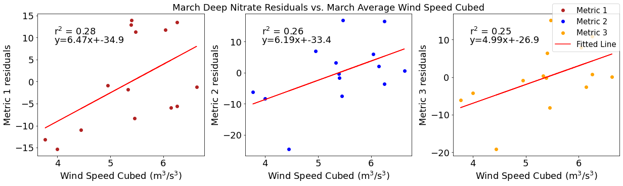
[53]:
# ---------- Solar ---------
fig4,ax4=plt.subplots(1,3,figsize=(17,5),constrained_layout=True)
ax4[0].plot(solarmar,deepno3resid1,'o',color='firebrick',label='Metric 1')
ax4[0].set_xlabel('Solar Irradiance (W/$\mathregular{m^2}$)')
ax4[0].set_ylabel('Metric 1 residuals')
y,r2,m,b=bloomdrivers.reg_r2(solarmar,deepno3resid1)
ax4[0].plot(solarmar, y, 'r')
ax4[0].text(0.1, 0.85, '$\mathregular{r^2}$ = %.2f'%r2, transform=ax4[0].transAxes)
ax4[0].text(0.1,0.78,f'y={round(m,2)}x+{round(b,1)}',horizontalalignment='left',verticalalignment='bottom',transform=ax4[0].transAxes)

ax4[1].plot(solarmar,deepno3resid2,'o',color='b',label='Metric 2')
ax4[1].set_xlabel('Solar Irradiance (W/$\mathregular{m^2}$)')
ax4[1].set_ylabel('Metric 2 residuals')
ax4[1].set_title('March Deep Nitrate Residuals vs. March Average Solar Radiation')
y,r2,m,b=bloomdrivers.reg_r2(solarmar,deepno3resid2)
ax4[1].plot(solarmar, y, 'r')
ax4[1].text(0.1, 0.85, '$\mathregular{r^2}$ = %.2f'%r2, transform=ax4[1].transAxes)
ax4[1].text(0.1,0.78,f'y={round(m,2)}x+{round(b,1)}',horizontalalignment='left',verticalalignment='bottom',transform=ax4[1].transAxes)

ax4[2].plot(solarmar,deepno3resid3,'o',color='orange',label='Metric 3')
ax4[2].set_xlabel('Solar Irradiance (W/$\mathregular{m^2}$)')
ax4[2].set_ylabel('Metric 3 residuals')
y,r2,m,b=bloomdrivers.reg_r2(solarmar,deepno3resid3)
ax4[2].plot(solarmar, y, 'r', label='Fitted Line')
ax4[2].text(0.1, 0.85, '$\mathregular{r^2}$ = %.2f'%r2, transform=ax4[2].transAxes)
ax4[2].text(0.1,0.78,f'y={round(m,2)}x+{round(b,1)}',horizontalalignment='left',verticalalignment='bottom',transform=ax4[2].transAxes)
fig4.legend()
[53]:
<matplotlib.legend.Legend at 0x7f652977a040>
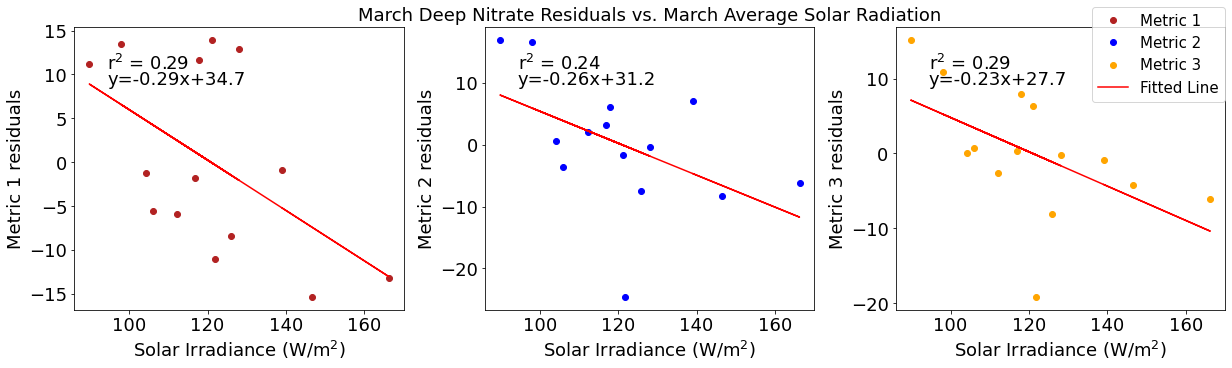
[54]:
# ---------- Temperature ---------
fig4,ax4=plt.subplots(1,3,figsize=(17,5),constrained_layout=True)
ax4[0].plot(tempmar,deepno3resid1,'o',color='firebrick',label='Metric 1')
ax4[0].set_xlabel('Surface Temperature ($^\circ$C)')
ax4[0].set_ylabel('Metric 1 residuals')
y,r2,m,b=bloomdrivers.reg_r2(tempmar,deepno3resid1)
ax4[0].plot(tempmar, y, 'r')
ax4[0].text(0.1, 0.85, '$\mathregular{r^2}$ = %.2f'%r2, transform=ax4[0].transAxes)
ax4[0].text(0.1,0.78,f'y={round(m,2)}x+{round(b,1)}',horizontalalignment='left',verticalalignment='bottom',transform=ax4[0].transAxes)

ax4[1].plot(tempmar,deepno3resid2,'o',color='b',label='Metric 2')
ax4[1].set_xlabel('Surface Temperature ($^\circ$C)')
ax4[1].set_ylabel('Metric 2 residuals')
ax4[1].set_title('March Deep Nitrate Residuals vs. March Average Surface Temperature')
y,r2,m,b=bloomdrivers.reg_r2(tempmar,deepno3resid2)
ax4[1].plot(tempmar, y, 'r')
ax4[1].text(0.1, 0.85, '$\mathregular{r^2}$ = %.2f'%r2, transform=ax4[1].transAxes)
ax4[1].text(0.1,0.78,f'y={round(m,2)}x+{round(b,1)}',horizontalalignment='left',verticalalignment='bottom',transform=ax4[1].transAxes)

ax4[2].plot(tempmar,deepno3resid3,'o',color='orange',label='Metric 3')
ax4[2].set_xlabel('Surface Temperature ($^\circ$C)')
ax4[2].set_ylabel('Metric 3 residuals')
y,r2,m,b=bloomdrivers.reg_r2(tempmar,deepno3resid3)
ax4[2].plot(tempmar, y, 'r', label='Fitted Line')
ax4[2].text(0.1, 0.85, '$\mathregular{r^2}$ = %.2f'%r2, transform=ax4[2].transAxes)
ax4[2].text(0.1,0.78,f'y={round(m,2)}x+{round(b,1)}',horizontalalignment='left',verticalalignment='bottom',transform=ax4[2].transAxes)
fig4.legend()
[54]:
<matplotlib.legend.Legend at 0x7f6529614550>
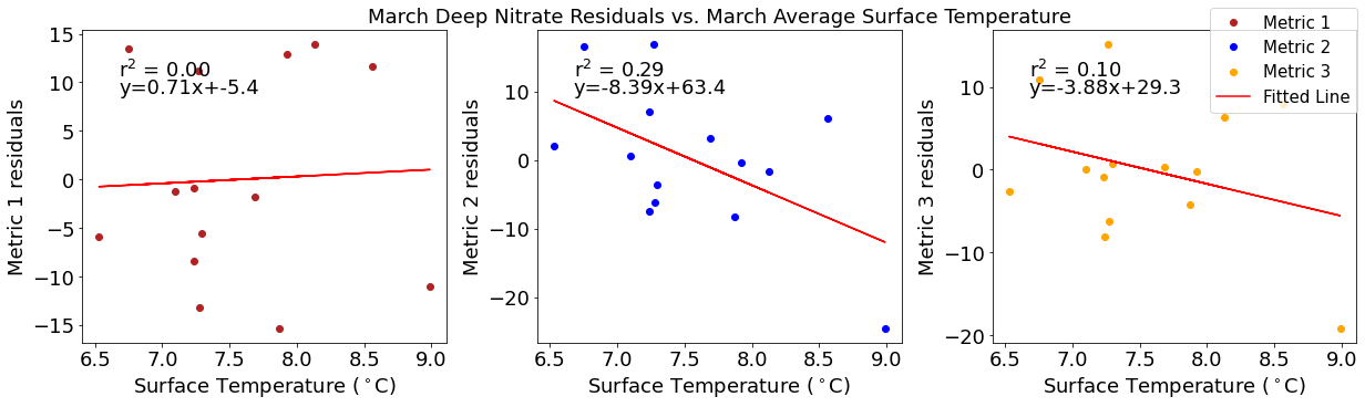
[55]:
# ---------- Deep NO3 ---------
fig4,ax4=plt.subplots(1,3,figsize=(17,5),constrained_layout=True)
ax4[0].plot(midno3mar,deepno3resid1,'o',color='firebrick',label='Metric 1')
ax4[0].set_xlabel('Concentration ($\mu$M N)')
ax4[0].set_ylabel('Metric 1 residuals')
y,r2,m,b=bloomdrivers.reg_r2(midno3mar,deepno3resid1)
ax4[0].plot(midno3mar, y, 'r')
ax4[0].text(0.1, 0.85, '$\mathregular{r^2}$ = %.2f'%r2, transform=ax4[0].transAxes)
ax4[0].text(0.1,0.78,f'y={round(m,2)}x+{round(b,1)}',horizontalalignment='left',verticalalignment='bottom',transform=ax4[0].transAxes)

ax4[1].plot(midno3mar,deepno3resid2,'o',color='b',label='Metric 2')
ax4[1].set_xlabel('Concentration ($\mu$M N)')
ax4[1].set_ylabel('Metric 2 residuals')
ax4[1].set_title('March Deep Nitrate Residuals vs. March Average Mid-depth Nitrate (30-90m)')
y,r2,m,b=bloomdrivers.reg_r2(midno3mar,deepno3resid2)
ax4[1].plot(midno3mar, y, 'r')
ax4[1].text(0.1, 0.85, '$\mathregular{r^2}$ = %.2f'%r2, transform=ax4[1].transAxes)
ax4[1].text(0.1,0.78,f'y={round(m,2)}x+{round(b,1)}',horizontalalignment='left',verticalalignment='bottom',transform=ax4[1].transAxes)

ax4[2].plot(midno3mar,deepno3resid3,'o',color='orange',label='Metric 3')
ax4[2].set_xlabel('Concentration ($\mu$M N)')
ax4[2].set_ylabel('Metric 3 residuals')
y,r2,m,b=bloomdrivers.reg_r2(midno3mar,deepno3resid3)
ax4[2].plot(midno3mar, y, 'r', label='Fitted Line')
ax4[2].text(0.1, 0.85, '$\mathregular{r^2}$ = %.2f'%r2, transform=ax4[2].transAxes)
ax4[2].text(0.1,0.78,f'y={round(m,2)}x+{round(b,1)}',horizontalalignment='left',verticalalignment='bottom',transform=ax4[2].transAxes)
fig4.legend()
[55]:
<matplotlib.legend.Legend at 0x7f65295fe730>
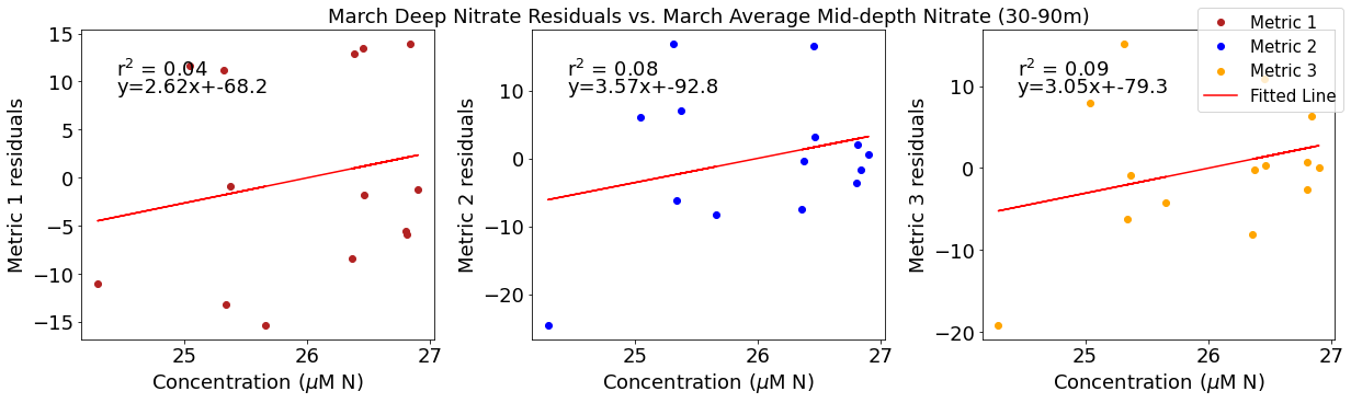
[56]:
# ---------- Salinity ---------
fig4,ax4=plt.subplots(1,3,figsize=(17,5),constrained_layout=True)
ax4[0].plot(salmar,deepno3resid1,'o',color='firebrick',label='Metric 1')
ax4[0].set_xlabel('Salinity (g/kg)')
ax4[0].set_ylabel('Metric 1 residuals')
y,r2,m,b=bloomdrivers.reg_r2(salmar,deepno3resid1)
ax4[0].plot(salmar, y, 'r')
ax4[0].text(0.1, 0.85, '$\mathregular{r^2}$ = %.2f'%r2, transform=ax4[0].transAxes)
ax4[0].text(0.1,0.78,f'y={round(m,2)}x+{round(b,1)}',horizontalalignment='left',verticalalignment='bottom',transform=ax4[0].transAxes)

ax4[1].plot(salmar,deepno3resid2,'o',color='b',label='Metric 2')
ax4[1].set_xlabel('Salinity (g/kg)')
ax4[1].set_ylabel('Metric 2 residuals')
ax4[1].set_title('March Deep Nitrate Residuals vs. March Average Absolute Surface Salinity')
y,r2,m,b=bloomdrivers.reg_r2(salmar,deepno3resid2)
ax4[1].plot(salmar, y, 'r')
ax4[1].text(0.1, 0.85, '$\mathregular{r^2}$ = %.2f'%r2, transform=ax4[1].transAxes)
ax4[1].text(0.1,0.78,f'y={round(m,2)}x+{round(b,1)}',horizontalalignment='left',verticalalignment='bottom',transform=ax4[1].transAxes)

ax4[2].plot(salmar,deepno3resid3,'o',color='orange',label='Metric 3')
ax4[2].set_xlabel('Salinity (g/kg)')
ax4[2].set_ylabel('Metric 3 residuals')
y,r2,m,b=bloomdrivers.reg_r2(salmar,deepno3resid3)
ax4[2].plot(salmar, y, 'r', label='Fitted Line')
ax4[2].text(0.1, 0.85, '$\mathregular{r^2}$ = %.2f'%r2, transform=ax4[2].transAxes)
ax4[2].text(0.1,0.78,f'y={round(m,2)}x+{round(b,1)}',horizontalalignment='left',verticalalignment='bottom',transform=ax4[2].transAxes)
fig4.legend()
[56]:
<matplotlib.legend.Legend at 0x7f6529494220>
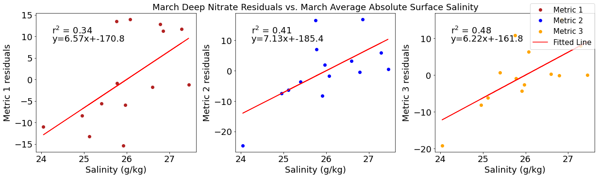
[57]:
# ---------- Fraser ---------
fig4,ax4=plt.subplots(1,3,figsize=(17,5),constrained_layout=True)
ax4[0].plot(frasermar,deepno3resid1,'o',color='firebrick',label='Metric 1')
ax4[0].set_xlabel('Flow (m$^3$s$^{-1}$)')
ax4[0].set_ylabel('Metric 1 residuals')
y,r2,m,b=bloomdrivers.reg_r2(frasermar,deepno3resid1)
ax4[0].plot(frasermar, y, 'r')
ax4[0].text(0.1, 0.85, '$\mathregular{r^2}$ = %.2f'%r2, transform=ax4[0].transAxes)
ax4[0].text(0.1,0.78,f'y={round(m,2)}x+{round(b,1)}',horizontalalignment='left',verticalalignment='bottom',transform=ax4[0].transAxes)

ax4[1].plot(frasermar,deepno3resid2,'o',color='b',label='Metric 2')
ax4[1].set_xlabel('Flow (m$^3$s$^{-1}$)')
ax4[1].set_ylabel('Metric 2 residuals')
ax4[1].set_title('March Deep Nitrate Residuals vs. March Average Fraser Flow')
y,r2,m,b=bloomdrivers.reg_r2(frasermar,deepno3resid2)
ax4[1].plot(frasermar, y, 'r')
ax4[1].text(0.1, 0.85, '$\mathregular{r^2}$ = %.2f'%r2, transform=ax4[1].transAxes)
ax4[1].text(0.1,0.78,f'y={round(m,2)}x+{round(b,1)}',horizontalalignment='left',verticalalignment='bottom',transform=ax4[1].transAxes)

ax4[2].plot(frasermar,deepno3resid3,'o',color='orange',label='Metric 3')
ax4[2].set_xlabel('Flow (m$^3$s$^{-1}$)')
ax4[2].set_ylabel('Metric 3 residuals')
y,r2,m,b=bloomdrivers.reg_r2(frasermar,deepno3resid3)
ax4[2].plot(frasermar, y, 'r', label='Fitted Line')
ax4[2].text(0.1, 0.85, '$\mathregular{r^2}$ = %.2f'%r2, transform=ax4[2].transAxes)
ax4[2].text(0.1,0.78,f'y={round(m,2)}x+{round(b,1)}',horizontalalignment='left',verticalalignment='bottom',transform=ax4[2].transAxes)
fig4.legend()
[57]:
<matplotlib.legend.Legend at 0x7f6529342190>
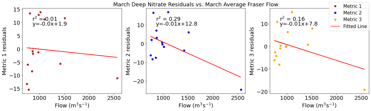
[58]:
# ---------- Halocline ---------
fig4,ax4=plt.subplots(1,3,figsize=(17,5),constrained_layout=True)
ax4[0].plot(halomar,deepno3resid1,'o',color='firebrick',label='Metric 1')
ax4[0].set_xlabel('Halocline Depth (m)')
ax4[0].set_ylabel('Metric 1 residuals')
y,r2,m,b=bloomdrivers.reg_r2(halomar,deepno3resid1)
ax4[0].plot(halomar, y, 'r')
ax4[0].text(0.1, 0.85, '$\mathregular{r^2}$ = %.2f'%r2, transform=ax4[0].transAxes)
ax4[0].text(0.1,0.78,f'y={round(m,2)}x+{round(b,1)}',horizontalalignment='left',verticalalignment='bottom',transform=ax4[0].transAxes)

ax4[1].plot(halomar,deepno3resid2,'o',color='b',label='Metric 2')
ax4[1].set_xlabel('Halocline Depth (m)')
ax4[1].set_ylabel('Metric 2 residuals')
ax4[1].set_title('March Deep Nitrate Residuals vs. March Halocline Depth')
y,r2,m,b=bloomdrivers.reg_r2(halomar,deepno3resid2)
ax4[1].plot(halomar, y, 'r')
ax4[1].text(0.1, 0.85, '$\mathregular{r^2}$ = %.2f'%r2, transform=ax4[1].transAxes)
ax4[1].text(0.1,0.78,f'y={round(m,2)}x+{round(b,1)}',horizontalalignment='left',verticalalignment='bottom',transform=ax4[1].transAxes)

ax4[2].plot(halomar,deepno3resid3,'o',color='orange',label='Metric 3')
ax4[2].set_xlabel('Halocline Depth (m)')
ax4[2].set_ylabel('Metric 3 residuals')
y,r2,m,b=bloomdrivers.reg_r2(halomar,deepno3resid3)
ax4[2].plot(halomar, y, 'r', label='Fitted Line')
ax4[2].text(0.1, 0.85, '$\mathregular{r^2}$ = %.2f'%r2, transform=ax4[2].transAxes)
ax4[2].text(0.1,0.78,f'y={round(m,2)}x+{round(b,1)}',horizontalalignment='left',verticalalignment='bottom',transform=ax4[2].transAxes)
fig4.legend()
[58]:
<matplotlib.legend.Legend at 0x7f65292701c0>
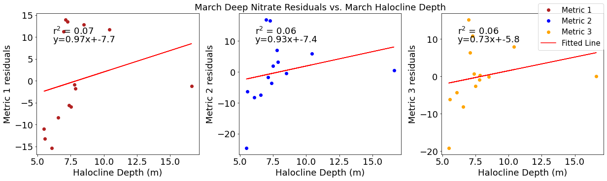
Correlation plots of salinity residuals
[59]:
#  residual calculations for each metric
salresid1=list()
y,r2,m,b=bloomdrivers.reg_r2(salmar,yearday1)
for ind,y in enumerate(yearday1):
    x=salmar[ind]
    salresid1.append(y-(m*x+b))

salresid2=list()
y,r2,m,b=bloomdrivers.reg_r2(salmar,yearday2)
for ind,y in enumerate(yearday2):
    x=salmar[ind]
    salresid2.append(y-(m*x+b))

salresid3=list()
y,r2,m,b=bloomdrivers.reg_r2(salmar,yearday3)
for ind,y in enumerate(yearday3):
    x=salmar[ind]
    salresid3.append(y-(m*x+b))
[60]:
dfsal=pd.DataFrame({'sal':salmar,'salresid1':salresid1,'salresid2':salresid2,'salresid3':salresid3,'wind':windmar,'solar':solarmar,
                    'temp':tempmar,'fraser':frasermar,'midno3':midno3mar,'deepno3':deepno3mar,'halocine':halomar})
[61]:
plt.subplots(figsize=(20,15))
cm1=cmocean.cm.curl
sns.heatmap(dfsal.corr(), annot = True,cmap=cm1,vmin=-1,vmax=1)
[61]:
<AxesSubplot:>
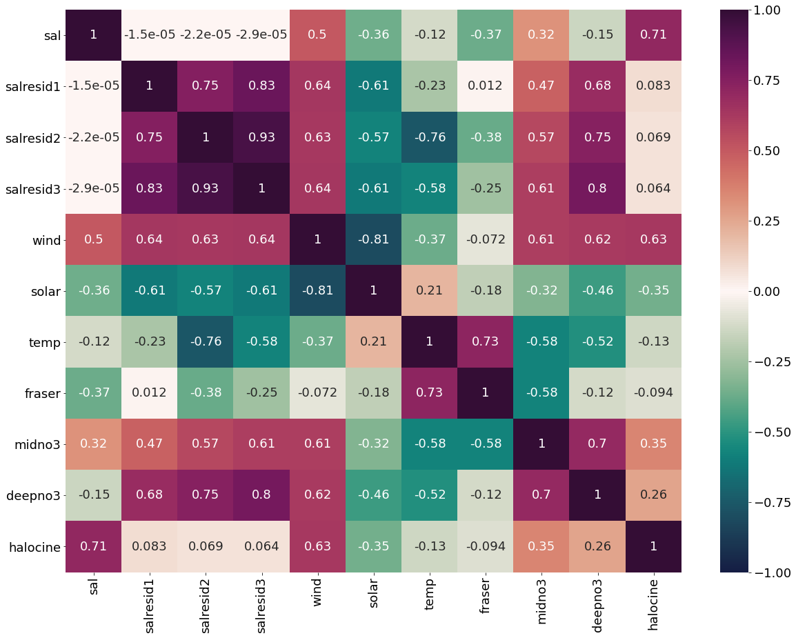
[62]:
# ---------- wind ---------
fig4,ax4=plt.subplots(1,3,figsize=(17,5),constrained_layout=True)
ax4[0].plot(windmar,salresid1,'o',color='firebrick',label='Metric 1')
ax4[0].set_xlabel('Wind Speed Cubed ($\mathregular{m^3}$/$\mathregular{s^3}$)')
ax4[0].set_ylabel('Metric 1 residuals')
y,r2,m,b=bloomdrivers.reg_r2(windmar,salresid1)
ax4[0].plot(windmar, y, 'r')
ax4[0].text(0.1, 0.85, '$\mathregular{r^2}$ = %.2f'%r2, transform=ax4[0].transAxes)
ax4[0].text(0.1,0.78,f'y={round(m,2)}x+{round(b,1)}',horizontalalignment='left',verticalalignment='bottom',transform=ax4[0].transAxes)

ax4[1].plot(windmar,salresid2,'o',color='b',label='Metric 2')
ax4[1].set_xlabel('Wind Speed Cubed ($\mathregular{m^3}$/$\mathregular{s^3}$)')
ax4[1].set_ylabel('Metric 2 residuals')
ax4[1].set_title('March Salinity Residuals vs. March Average Wind Speed Cubed')
y,r2,m,b=bloomdrivers.reg_r2(windmar,salresid2)
ax4[1].plot(windmar, y, 'r')
ax4[1].text(0.1, 0.85, '$\mathregular{r^2}$ = %.2f'%r2, transform=ax4[1].transAxes)
ax4[1].text(0.1,0.78,f'y={round(m,2)}x+{round(b,1)}',horizontalalignment='left',verticalalignment='bottom',transform=ax4[1].transAxes)

ax4[2].plot(windmar,salresid3,'o',color='orange',label='Metric 3')
ax4[2].set_xlabel('Wind Speed Cubed ($\mathregular{m^3}$/$\mathregular{s^3}$)')
ax4[2].set_ylabel('Metric 3 residuals')
y,r2,m,b=bloomdrivers.reg_r2(windmar,salresid3)
ax4[2].plot(windmar, y, 'r', label='Fitted Line')
ax4[2].text(0.1, 0.85, '$\mathregular{r^2}$ = %.2f'%r2, transform=ax4[2].transAxes)
ax4[2].text(0.1,0.78,f'y={round(m,2)}x+{round(b,1)}',horizontalalignment='left',verticalalignment='bottom',transform=ax4[2].transAxes)
fig4.legend()
[62]:
<matplotlib.legend.Legend at 0x7f6528f9e1f0>
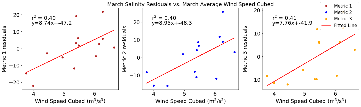
[63]:
# ---------- Solar ---------
fig4,ax4=plt.subplots(1,3,figsize=(17,5),constrained_layout=True)
ax4[0].plot(solarmar,salresid1,'o',color='firebrick',label='Metric 1')
ax4[0].set_xlabel('Solar Irradiance (W/$\mathregular{m^2}$)')
ax4[0].set_ylabel('Metric 1 residuals')
y,r2,m,b=bloomdrivers.reg_r2(solarmar,salresid1)
ax4[0].plot(solarmar, y, 'r')
ax4[0].text(0.1, 0.85, '$\mathregular{r^2}$ = %.2f'%r2, transform=ax4[0].transAxes)
ax4[0].text(0.1,0.78,f'y={round(m,2)}x+{round(b,1)}',horizontalalignment='left',verticalalignment='bottom',transform=ax4[0].transAxes)

ax4[1].plot(solarmar,salresid2,'o',color='b',label='Metric 2')
ax4[1].set_xlabel('Solar Irradiance (W/$\mathregular{m^2}$)')
ax4[1].set_ylabel('Metric 2 residuals')
ax4[1].set_title('March Salinity Residuals vs. March Average Solar Radiation')
y,r2,m,b=bloomdrivers.reg_r2(solarmar,salresid2)
ax4[1].plot(solarmar, y, 'r')
ax4[1].text(0.1, 0.85, '$\mathregular{r^2}$ = %.2f'%r2, transform=ax4[1].transAxes)
ax4[1].text(0.1,0.78,f'y={round(m,2)}x+{round(b,1)}',horizontalalignment='left',verticalalignment='bottom',transform=ax4[1].transAxes)

ax4[2].plot(solarmar,salresid3,'o',color='orange',label='Metric 3')
ax4[2].set_xlabel('Solar Irradiance (W/$\mathregular{m^2}$)')
ax4[2].set_ylabel('Metric 3 residuals')
y,r2,m,b=bloomdrivers.reg_r2(solarmar,salresid3)
ax4[2].plot(solarmar, y, 'r', label='Fitted Line')
ax4[2].text(0.1, 0.85, '$\mathregular{r^2}$ = %.2f'%r2, transform=ax4[2].transAxes)
ax4[2].text(0.1,0.78,f'y={round(m,2)}x+{round(b,1)}',horizontalalignment='left',verticalalignment='bottom',transform=ax4[2].transAxes)
fig4.legend()
[63]:
<matplotlib.legend.Legend at 0x7f6528eaf850>
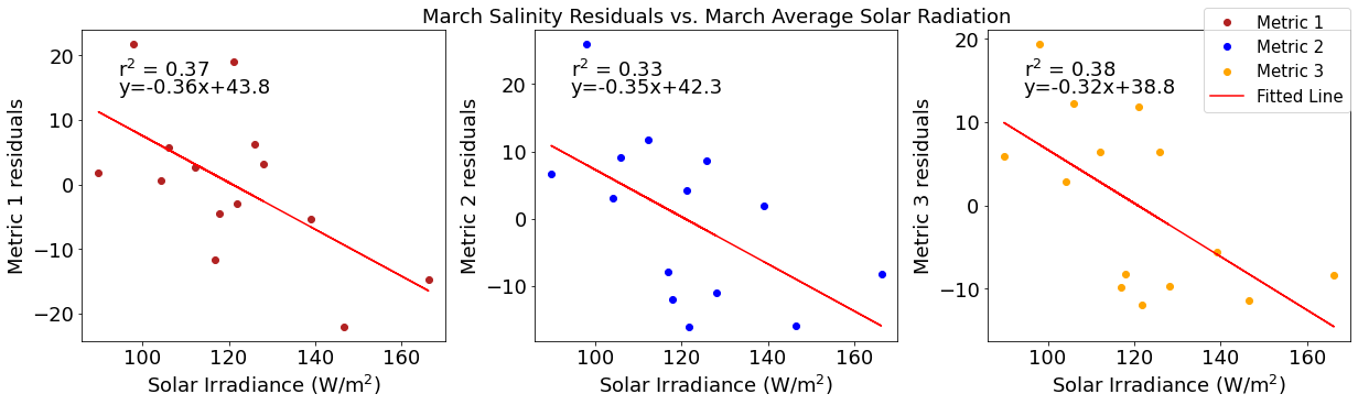
[64]:
# ---------- Temperature ---------
fig4,ax4=plt.subplots(1,3,figsize=(17,5),constrained_layout=True)
ax4[0].plot(tempmar,salresid1,'o',color='firebrick',label='Metric 1')
ax4[0].set_xlabel('Surface Temperature ($^\circ$C)')
ax4[0].set_ylabel('Metric 1 residuals')
y,r2,m,b=bloomdrivers.reg_r2(tempmar,salresid1)
ax4[0].plot(tempmar, y, 'r')
ax4[0].text(0.1, 0.85, '$\mathregular{r^2}$ = %.2f'%r2, transform=ax4[0].transAxes)
ax4[0].text(0.1,0.78,f'y={round(m,2)}x+{round(b,1)}',horizontalalignment='left',verticalalignment='bottom',transform=ax4[0].transAxes)

ax4[1].plot(tempmar,salresid2,'o',color='b',label='Metric 2')
ax4[1].set_xlabel('Surface Temperature ($^\circ$C)')
ax4[1].set_ylabel('Metric 2 residuals')
ax4[1].set_title('March Salinity Residuals vs. March Average Surface Temperature')
y,r2,m,b=bloomdrivers.reg_r2(tempmar,salresid2)
ax4[1].plot(tempmar, y, 'r')
ax4[1].text(0.1, 0.85, '$\mathregular{r^2}$ = %.2f'%r2, transform=ax4[1].transAxes)
ax4[1].text(0.1,0.78,f'y={round(m,2)}x+{round(b,1)}',horizontalalignment='left',verticalalignment='bottom',transform=ax4[1].transAxes)

ax4[2].plot(tempmar,salresid3,'o',color='orange',label='Metric 3')
ax4[2].set_xlabel('Surface Temperature ($^\circ$C)')
ax4[2].set_ylabel('Metric 3 residuals')
y,r2,m,b=bloomdrivers.reg_r2(tempmar,salresid3)
ax4[2].plot(tempmar, y, 'r', label='Fitted Line')
ax4[2].text(0.1, 0.85, '$\mathregular{r^2}$ = %.2f'%r2, transform=ax4[2].transAxes)
ax4[2].text(0.1,0.78,f'y={round(m,2)}x+{round(b,1)}',horizontalalignment='left',verticalalignment='bottom',transform=ax4[2].transAxes)
fig4.legend()
[64]:
<matplotlib.legend.Legend at 0x7f6528d48dc0>
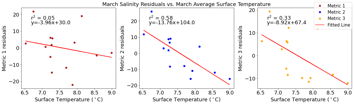
[65]:
# ---------- Deep NO3 ---------
fig4,ax4=plt.subplots(1,3,figsize=(17,5),constrained_layout=True)
ax4[0].plot(midno3mar,salresid1,'o',color='firebrick',label='Metric 1')
ax4[0].set_xlabel('Concentration ($\mu$M N)')
ax4[0].set_ylabel('Metric 1 residuals')
y,r2,m,b=bloomdrivers.reg_r2(midno3mar,salresid1)
ax4[0].plot(midno3mar, y, 'r')
ax4[0].text(0.1, 0.85, '$\mathregular{r^2}$ = %.2f'%r2, transform=ax4[0].transAxes)
ax4[0].text(0.1,0.78,f'y={round(m,2)}x+{round(b,1)}',horizontalalignment='left',verticalalignment='bottom',transform=ax4[0].transAxes)

ax4[1].plot(midno3mar,salresid2,'o',color='b',label='Metric 2')
ax4[1].set_xlabel('Concentration ($\mu$M N)')
ax4[1].set_ylabel('Metric 2 residuals')
ax4[1].set_title('March Salinity Residuals vs. March Average Mid-depth Nitrate (30-90m)')
y,r2,m,b=bloomdrivers.reg_r2(midno3mar,salresid2)
ax4[1].plot(midno3mar, y, 'r')
ax4[1].text(0.1, 0.85, '$\mathregular{r^2}$ = %.2f'%r2, transform=ax4[1].transAxes)
ax4[1].text(0.1,0.78,f'y={round(m,2)}x+{round(b,1)}',horizontalalignment='left',verticalalignment='bottom',transform=ax4[1].transAxes)

ax4[2].plot(midno3mar,salresid3,'o',color='orange',label='Metric 3')
ax4[2].set_xlabel('Concentration ($\mu$M N)')
ax4[2].set_ylabel('Metric 3 residuals')
y,r2,m,b=bloomdrivers.reg_r2(midno3mar,salresid3)
ax4[2].plot(midno3mar, y, 'r', label='Fitted Line')
ax4[2].text(0.1, 0.85, '$\mathregular{r^2}$ = %.2f'%r2, transform=ax4[2].transAxes)
ax4[2].text(0.1,0.78,f'y={round(m,2)}x+{round(b,1)}',horizontalalignment='left',verticalalignment='bottom',transform=ax4[2].transAxes)
fig4.legend()
[65]:
<matplotlib.legend.Legend at 0x7f6528c74580>
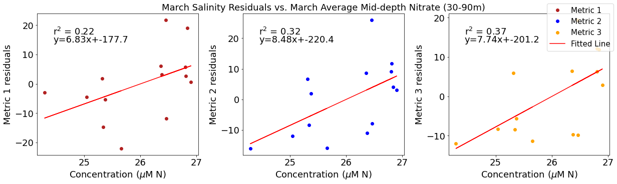
[66]:
# ---------- Deep NO3 ---------
fig4,ax4=plt.subplots(1,3,figsize=(17,5),constrained_layout=True)
ax4[0].plot(deepno3mar,salresid1,'o',color='firebrick',label='Metric 1')
ax4[0].set_xlabel('Concentration ($\mu$M N)')
ax4[0].set_ylabel('Metric 1 residuals')
y,r2,m,b=bloomdrivers.reg_r2(deepno3mar,salresid1)
ax4[0].plot(deepno3mar, y, 'r')
ax4[0].text(0.1, 0.85, '$\mathregular{r^2}$ = %.2f'%r2, transform=ax4[0].transAxes)
ax4[0].text(0.1,0.78,f'y={round(m,2)}x+{round(b,1)}',horizontalalignment='left',verticalalignment='bottom',transform=ax4[0].transAxes)

ax4[1].plot(deepno3mar,salresid2,'o',color='b',label='Metric 2')
ax4[1].set_xlabel('Concentration ($\mu$M N)')
ax4[1].set_ylabel('Metric 2 residuals')
ax4[1].set_title('March Salinity Residuals vs. March Average Deep Nitrate (below 250m)')
y,r2,m,b=bloomdrivers.reg_r2(deepno3mar,salresid2)
ax4[1].plot(deepno3mar, y, 'r')
ax4[1].text(0.1, 0.85, '$\mathregular{r^2}$ = %.2f'%r2, transform=ax4[1].transAxes)
ax4[1].text(0.1,0.78,f'y={round(m,2)}x+{round(b,1)}',horizontalalignment='left',verticalalignment='bottom',transform=ax4[1].transAxes)

ax4[2].plot(deepno3mar,salresid3,'o',color='orange',label='Metric 3')
ax4[2].set_xlabel('Concentration ($\mu$M N)')
ax4[2].set_ylabel('Metric 3 residuals')
y,r2,m,b=bloomdrivers.reg_r2(deepno3mar,salresid3)
ax4[2].plot(deepno3mar, y, 'r', label='Fitted Line')
ax4[2].text(0.1, 0.85, '$\mathregular{r^2}$ = %.2f'%r2, transform=ax4[2].transAxes)
ax4[2].text(0.1,0.78,f'y={round(m,2)}x+{round(b,1)}',horizontalalignment='left',verticalalignment='bottom',transform=ax4[2].transAxes)
fig4.legend()
[66]:
<matplotlib.legend.Legend at 0x7f6528b0d2e0>
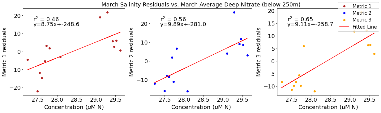
[67]:
# ---------- Fraser ---------
fig4,ax4=plt.subplots(1,3,figsize=(17,5),constrained_layout=True)
ax4[0].plot(frasermar,salresid1,'o',color='firebrick',label='Metric 1')
ax4[0].set_xlabel('Flow (m$^3$s$^{-1}$)')
ax4[0].set_ylabel('Metric 1 residuals')
y,r2,m,b=bloomdrivers.reg_r2(frasermar,salresid1)
ax4[0].plot(frasermar, y, 'r')
ax4[0].text(0.1, 0.85, '$\mathregular{r^2}$ = %.2f'%r2, transform=ax4[0].transAxes)
ax4[0].text(0.1,0.78,f'y={round(m,2)}x+{round(b,1)}',horizontalalignment='left',verticalalignment='bottom',transform=ax4[0].transAxes)

ax4[1].plot(frasermar,salresid2,'o',color='b',label='Metric 2')
ax4[1].set_xlabel('Flow (m$^3$s$^{-1}$)')
ax4[1].set_ylabel('Metric 2 residuals')
ax4[1].set_title('March Salinity Residuals vs. March Average Fraser Flow')
y,r2,m,b=bloomdrivers.reg_r2(frasermar,salresid2)
ax4[1].plot(frasermar, y, 'r')
ax4[1].text(0.1, 0.85, '$\mathregular{r^2}$ = %.2f'%r2, transform=ax4[1].transAxes)
ax4[1].text(0.1,0.78,f'y={round(m,2)}x+{round(b,1)}',horizontalalignment='left',verticalalignment='bottom',transform=ax4[1].transAxes)

ax4[2].plot(frasermar,salresid3,'o',color='orange',label='Metric 3')
ax4[2].set_xlabel('Flow (m$^3$s$^{-1}$)')
ax4[2].set_ylabel('Metric 3 residuals')
y,r2,m,b=bloomdrivers.reg_r2(frasermar,salresid3)
ax4[2].plot(frasermar, y, 'r', label='Fitted Line')
ax4[2].text(0.1, 0.85, '$\mathregular{r^2}$ = %.2f'%r2, transform=ax4[2].transAxes)
ax4[2].text(0.1,0.78,f'y={round(m,2)}x+{round(b,1)}',horizontalalignment='left',verticalalignment='bottom',transform=ax4[2].transAxes)
fig4.legend()
[67]:
<matplotlib.legend.Legend at 0x7f6528a29a30>
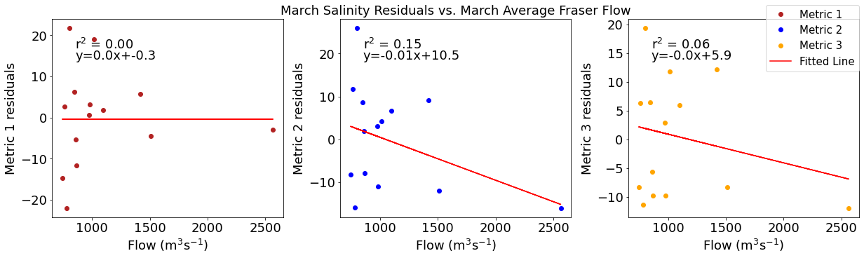
[68]:
# ---------- Halocline ---------
fig4,ax4=plt.subplots(1,3,figsize=(17,5),constrained_layout=True)
ax4[0].plot(halomar,salresid1,'o',color='firebrick',label='Metric 1')
ax4[0].set_xlabel('Halocline Depth (m)')
ax4[0].set_ylabel('Metric 1 residuals')
y,r2,m,b=bloomdrivers.reg_r2(halomar,salresid1)
ax4[0].plot(halomar, y, 'r')
ax4[0].text(0.1, 0.85, '$\mathregular{r^2}$ = %.2f'%r2, transform=ax4[0].transAxes)
ax4[0].text(0.1,0.78,f'y={round(m,2)}x+{round(b,1)}',horizontalalignment='left',verticalalignment='bottom',transform=ax4[0].transAxes)

ax4[1].plot(halomar,salresid2,'o',color='b',label='Metric 2')
ax4[1].set_xlabel('Halocline Depth (m)')
ax4[1].set_ylabel('Metric 2 residuals')
ax4[1].set_title('March Salinity Residuals vs. March Halocline Depth')
y,r2,m,b=bloomdrivers.reg_r2(halomar,salresid2)
ax4[1].plot(halomar, y, 'r')
ax4[1].text(0.1, 0.85, '$\mathregular{r^2}$ = %.2f'%r2, transform=ax4[1].transAxes)
ax4[1].text(0.1,0.78,f'y={round(m,2)}x+{round(b,1)}',horizontalalignment='left',verticalalignment='bottom',transform=ax4[1].transAxes)

ax4[2].plot(halomar,salresid3,'o',color='orange',label='Metric 3')
ax4[2].set_xlabel('Halocline Depth (m)')
ax4[2].set_ylabel('Metric 3 residuals')
y,r2,m,b=bloomdrivers.reg_r2(halomar,salresid3)
ax4[2].plot(halomar, y, 'r', label='Fitted Line')
ax4[2].text(0.1, 0.85, '$\mathregular{r^2}$ = %.2f'%r2, transform=ax4[2].transAxes)
ax4[2].text(0.1,0.78,f'y={round(m,2)}x+{round(b,1)}',horizontalalignment='left',verticalalignment='bottom',transform=ax4[2].transAxes)
fig4.legend()
[68]:
<matplotlib.legend.Legend at 0x7f65289bae20>
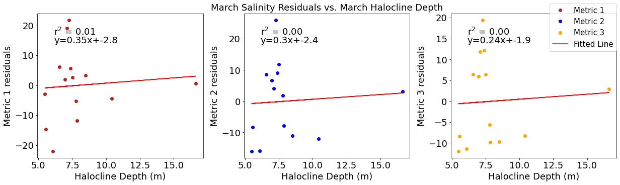
Correlation plots of Fraser flow residuals
[69]:
#  residual calculations for each metric
fraserresid1=list()
y,r2,m,b=bloomdrivers.reg_r2(frasermar,yearday1)
for ind,y in enumerate(yearday1):
    x=frasermar[ind]
    fraserresid1.append(y-(m*x+b))

fraserresid2=list()
y,r2,m,b=bloomdrivers.reg_r2(frasermar,yearday2)
for ind,y in enumerate(yearday2):
    x=frasermar[ind]
    fraserresid2.append(y-(m*x+b))

fraserresid3=list()
y,r2,m,b=bloomdrivers.reg_r2(frasermar,yearday3)
for ind,y in enumerate(yearday3):
    x=frasermar[ind]
    fraserresid3.append(y-(m*x+b))
[70]:
dffraser=pd.DataFrame({'fraser':frasermar,'fraserresid1':fraserresid1,'fraserresid2':fraserresid2,'fraserresid3':fraserresid3,'wind':windmar,'solar':solarmar,
                    'temp':tempmar,'midno3':midno3mar,'deepno3':deepno3mar,'halocine':halomar})
[71]:
plt.subplots(figsize=(20,15))
cm1=cmocean.cm.curl
sns.heatmap(dffraser.corr(), annot = True,cmap=cm1,vmin=-1,vmax=1)
[71]:
<AxesSubplot:>
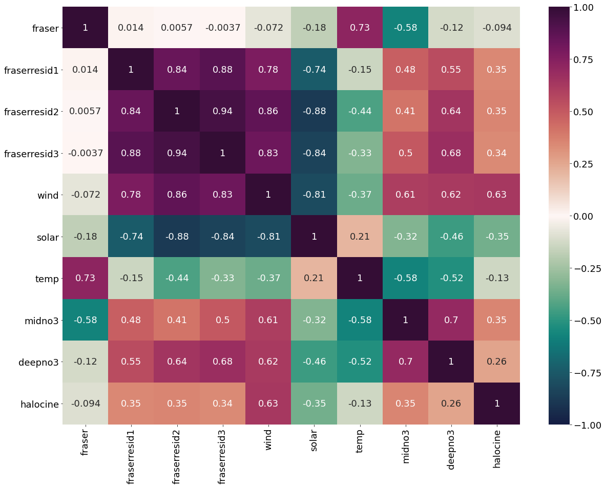
[72]:
# ---------- wind ---------
fig4,ax4=plt.subplots(1,3,figsize=(17,5),constrained_layout=True)
ax4[0].plot(windmar,fraserresid1,'o',color='firebrick',label='Metric 1')
ax4[0].set_xlabel('Wind Speed Cubed ($\mathregular{m^3}$/$\mathregular{s^3}$)')
ax4[0].set_ylabel('Metric 1 residuals')
y,r2,m,b=bloomdrivers.reg_r2(windmar,fraserresid1)
ax4[0].plot(windmar, y, 'r')
ax4[0].text(0.1, 0.85, '$\mathregular{r^2}$ = %.2f'%r2, transform=ax4[0].transAxes)
ax4[0].text(0.1,0.78,f'y={round(m,2)}x+{round(b,1)}',horizontalalignment='left',verticalalignment='bottom',transform=ax4[0].transAxes)

ax4[1].plot(windmar,fraserresid2,'o',color='b',label='Metric 2')
ax4[1].set_xlabel('Wind Speed Cubed ($\mathregular{m^3}$/$\mathregular{s^3}$)')
ax4[1].set_ylabel('Metric 2 residuals')
ax4[1].set_title('March Fraser Residuals vs. March Average Wind Speed Cubed')
y,r2,m,b=bloomdrivers.reg_r2(windmar,fraserresid2)
ax4[1].plot(windmar, y, 'r')
ax4[1].text(0.1, 0.85, '$\mathregular{r^2}$ = %.2f'%r2, transform=ax4[1].transAxes)
ax4[1].text(0.1,0.78,f'y={round(m,2)}x+{round(b,1)}',horizontalalignment='left',verticalalignment='bottom',transform=ax4[1].transAxes)

ax4[2].plot(windmar,fraserresid3,'o',color='orange',label='Metric 3')
ax4[2].set_xlabel('Wind Speed Cubed ($\mathregular{m^3}$/$\mathregular{s^3}$)')
ax4[2].set_ylabel('Metric 3 residuals')
y,r2,m,b=bloomdrivers.reg_r2(windmar,fraserresid3)
ax4[2].plot(windmar, y, 'r', label='Fitted Line')
ax4[2].text(0.1, 0.85, '$\mathregular{r^2}$ = %.2f'%r2, transform=ax4[2].transAxes)
ax4[2].text(0.1,0.78,f'y={round(m,2)}x+{round(b,1)}',horizontalalignment='left',verticalalignment='bottom',transform=ax4[2].transAxes)
fig4.legend()
[72]:
<matplotlib.legend.Legend at 0x7f6529417eb0>
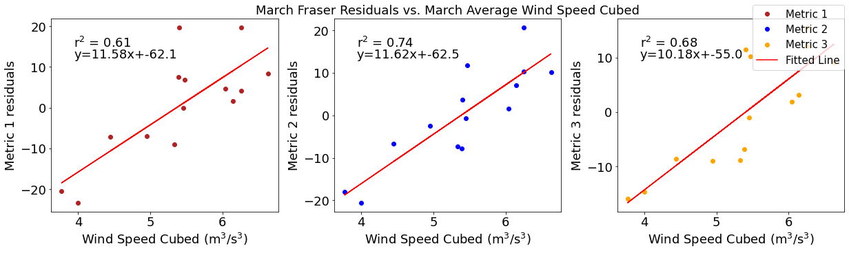
[73]:
# ---------- Solar ---------
fig4,ax4=plt.subplots(1,3,figsize=(17,5),constrained_layout=True)
ax4[0].plot(solarmar, fraserresid1,'o',color='firebrick',label='Metric 1')
ax4[0].set_xlabel('Solar Irradiance (W/$\mathregular{m^2}$)')
ax4[0].set_ylabel('Metric 1 residuals')
y,r2,m,b=bloomdrivers.reg_r2(solarmar,fraserresid1)
ax4[0].plot(solarmar, y, 'r')
ax4[0].text(0.1, 0.85, '$\mathregular{r^2}$ = %.2f'%r2, transform=ax4[0].transAxes)
ax4[0].text(0.1,0.78,f'y={round(m,2)}x+{round(b,1)}',horizontalalignment='left',verticalalignment='bottom',transform=ax4[0].transAxes)

ax4[1].plot(solarmar,fraserresid2,'o',color='b',label='Metric 2')
ax4[1].set_xlabel('Solar Irradiance (W/$\mathregular{m^2}$)')
ax4[1].set_ylabel('Metric 2 residuals')
ax4[1].set_title('March Fraser Residuals vs. March Average Solar Radiation')
y,r2,m,b=bloomdrivers.reg_r2(solarmar,fraserresid2)
ax4[1].plot(solarmar, y, 'r')
ax4[1].text(0.1, 0.85, '$\mathregular{r^2}$ = %.2f'%r2, transform=ax4[1].transAxes)
ax4[1].text(0.1,0.78,f'y={round(m,2)}x+{round(b,1)}',horizontalalignment='left',verticalalignment='bottom',transform=ax4[1].transAxes)

ax4[2].plot(solarmar,fraserresid3,'o',color='orange',label='Metric 3')
ax4[2].set_xlabel('Solar Irradiance (W/$\mathregular{m^2}$)')
ax4[2].set_ylabel('Metric 3 residuals')
y,r2,m,b=bloomdrivers.reg_r2(solarmar,fraserresid3)
ax4[2].plot(solarmar, y, 'r', label='Fitted Line')
ax4[2].text(0.1, 0.85, '$\mathregular{r^2}$ = %.2f'%r2, transform=ax4[2].transAxes)
ax4[2].text(0.1,0.78,f'y={round(m,2)}x+{round(b,1)}',horizontalalignment='left',verticalalignment='bottom',transform=ax4[2].transAxes)
fig4.legend()
[73]:
<matplotlib.legend.Legend at 0x7f6528656220>
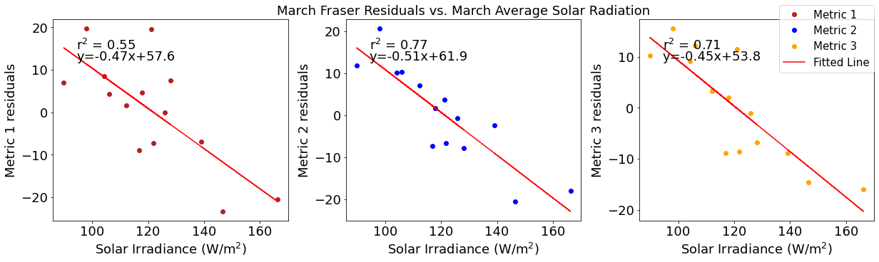
[74]:
# ---------- Temperature ---------
fig4,ax4=plt.subplots(1,3,figsize=(17,5),constrained_layout=True)
ax4[0].plot(tempmar,fraserresid1,'o',color='firebrick',label='Metric 1')
ax4[0].set_xlabel('Surface Temperature ($^\circ$C)')
ax4[0].set_ylabel('Metric 1 residuals')
y,r2,m,b=bloomdrivers.reg_r2(tempmar,fraserresid1)
ax4[0].plot(tempmar, y, 'r')
ax4[0].text(0.1, 0.85, '$\mathregular{r^2}$ = %.2f'%r2, transform=ax4[0].transAxes)
ax4[0].text(0.1,0.78,f'y={round(m,2)}x+{round(b,1)}',horizontalalignment='left',verticalalignment='bottom',transform=ax4[0].transAxes)

ax4[1].plot(tempmar,fraserresid2,'o',color='b',label='Metric 2')
ax4[1].set_xlabel('Surface Temperature ($^\circ$C)')
ax4[1].set_ylabel('Metric 2 residuals')
ax4[1].set_title('March Fraser Residuals vs. March Average Surface Temperature')
y,r2,m,b=bloomdrivers.reg_r2(tempmar,fraserresid2)
ax4[1].plot(tempmar, y, 'r')
ax4[1].text(0.1, 0.85, '$\mathregular{r^2}$ = %.2f'%r2, transform=ax4[1].transAxes)
ax4[1].text(0.1,0.78,f'y={round(m,2)}x+{round(b,1)}',horizontalalignment='left',verticalalignment='bottom',transform=ax4[1].transAxes)

ax4[2].plot(tempmar,fraserresid3,'o',color='orange',label='Metric 3')
ax4[2].set_xlabel('Surface Temperature ($^\circ$C)')
ax4[2].set_ylabel('Metric 3 residuals')
y,r2,m,b=bloomdrivers.reg_r2(tempmar,fraserresid3)
ax4[2].plot(tempmar, y, 'r', label='Fitted Line')
ax4[2].text(0.1, 0.85, '$\mathregular{r^2}$ = %.2f'%r2, transform=ax4[2].transAxes)
ax4[2].text(0.1,0.78,f'y={round(m,2)}x+{round(b,1)}',horizontalalignment='left',verticalalignment='bottom',transform=ax4[2].transAxes)
fig4.legend()
[74]:
<matplotlib.legend.Legend at 0x7f6528561790>
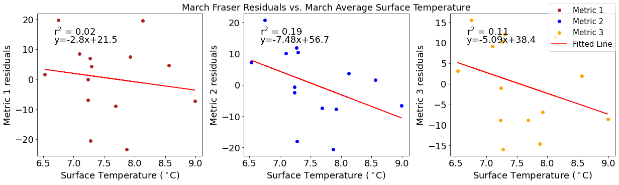
[75]:
# ---------- Deep NO3 ---------
fig4,ax4=plt.subplots(1,3,figsize=(17,5),constrained_layout=True)
ax4[0].plot(midno3mar,fraserresid1,'o',color='firebrick',label='Metric 1')
ax4[0].set_xlabel('Concentration ($\mu$M N)')
ax4[0].set_ylabel('Metric 1 residuals')
y,r2,m,b=bloomdrivers.reg_r2(midno3mar,fraserresid1)
ax4[0].plot(midno3mar, y, 'r')
ax4[0].text(0.1, 0.85, '$\mathregular{r^2}$ = %.2f'%r2, transform=ax4[0].transAxes)
ax4[0].text(0.1,0.78,f'y={round(m,2)}x+{round(b,1)}',horizontalalignment='left',verticalalignment='bottom',transform=ax4[0].transAxes)

ax4[1].plot(midno3mar,fraserresid2,'o',color='b',label='Metric 2')
ax4[1].set_xlabel('Concentration ($\mu$M N)')
ax4[1].set_ylabel('Metric 2 residuals')
ax4[1].set_title('March Fraser Residuals vs. March Average Mid-depth Nitrate (30-90m)')
y,r2,m,b=bloomdrivers.reg_r2(midno3mar,fraserresid2)
ax4[1].plot(midno3mar, y, 'r')
ax4[1].text(0.1, 0.85, '$\mathregular{r^2}$ = %.2f'%r2, transform=ax4[1].transAxes)
ax4[1].text(0.1,0.78,f'y={round(m,2)}x+{round(b,1)}',horizontalalignment='left',verticalalignment='bottom',transform=ax4[1].transAxes)

ax4[2].plot(midno3mar,fraserresid3,'o',color='orange',label='Metric 3')
ax4[2].set_xlabel('Concentration ($\mu$M N)')
ax4[2].set_ylabel('Metric 3 residuals')
y,r2,m,b=bloomdrivers.reg_r2(midno3mar,fraserresid3)
ax4[2].plot(midno3mar, y, 'r', label='Fitted Line')
ax4[2].text(0.1, 0.85, '$\mathregular{r^2}$ = %.2f'%r2, transform=ax4[2].transAxes)
ax4[2].text(0.1,0.78,f'y={round(m,2)}x+{round(b,1)}',horizontalalignment='left',verticalalignment='bottom',transform=ax4[2].transAxes)
fig4.legend()
[75]:
<matplotlib.legend.Legend at 0x7f6528474c10>
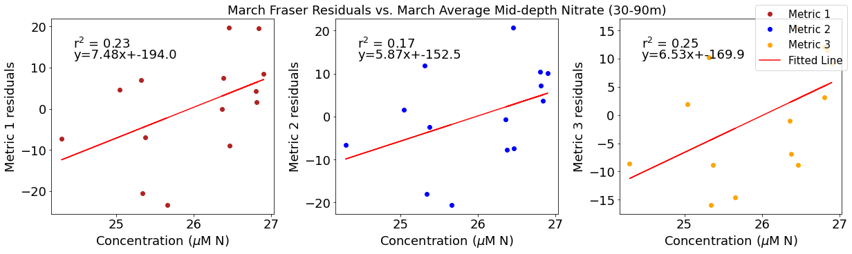
[76]:
# ---------- Deep NO3 ---------
fig4,ax4=plt.subplots(1,3,figsize=(17,5),constrained_layout=True)
ax4[0].plot(deepno3mar,fraserresid1,'o',color='firebrick',label='Metric 1')
ax4[0].set_xlabel('Concentration ($\mu$M N)')
ax4[0].set_ylabel('Metric 1 residuals')
y,r2,m,b=bloomdrivers.reg_r2(deepno3mar,fraserresid1)
ax4[0].plot(deepno3mar, y, 'r')
ax4[0].text(0.1, 0.85, '$\mathregular{r^2}$ = %.2f'%r2, transform=ax4[0].transAxes)
ax4[0].text(0.1,0.78,f'y={round(m,2)}x+{round(b,1)}',horizontalalignment='left',verticalalignment='bottom',transform=ax4[0].transAxes)

ax4[1].plot(deepno3mar,fraserresid2,'o',color='b',label='Metric 2')
ax4[1].set_xlabel('Concentration ($\mu$M N)')
ax4[1].set_ylabel('Metric 2 residuals')
ax4[1].set_title('March Fraser Residuals vs. March Average Deep Nitrate (below 250m)')
y,r2,m,b=bloomdrivers.reg_r2(deepno3mar,fraserresid2)
ax4[1].plot(deepno3mar, y, 'r')
ax4[1].text(0.1, 0.85, '$\mathregular{r^2}$ = %.2f'%r2, transform=ax4[1].transAxes)
ax4[1].text(0.1,0.78,f'y={round(m,2)}x+{round(b,1)}',horizontalalignment='left',verticalalignment='bottom',transform=ax4[1].transAxes)

ax4[2].plot(deepno3mar,fraserresid3,'o',color='orange',label='Metric 3')
ax4[2].set_xlabel('Concentration ($\mu$M N)')
ax4[2].set_ylabel('Metric 3 residuals')
y,r2,m,b=bloomdrivers.reg_r2(deepno3mar,fraserresid3)
ax4[2].plot(deepno3mar, y, 'r', label='Fitted Line')
ax4[2].text(0.1, 0.85, '$\mathregular{r^2}$ = %.2f'%r2, transform=ax4[2].transAxes)
ax4[2].text(0.1,0.78,f'y={round(m,2)}x+{round(b,1)}',horizontalalignment='left',verticalalignment='bottom',transform=ax4[2].transAxes)
fig4.legend()
[76]:
<matplotlib.legend.Legend at 0x7f652830ddf0>
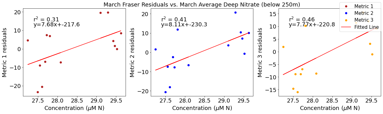
[77]:
# ---------- Salinity ---------
fig4,ax4=plt.subplots(1,3,figsize=(17,5),constrained_layout=True)
ax4[0].plot(salmar,fraserresid1,'o',color='firebrick',label='Metric 1')
ax4[0].set_xlabel('Salinity (g/kg)')
ax4[0].set_ylabel('Metric 1 residuals')
y,r2,m,b=bloomdrivers.reg_r2(salmar,fraserresid1)
ax4[0].plot(salmar, y, 'r')
ax4[0].text(0.1, 0.85, '$\mathregular{r^2}$ = %.2f'%r2, transform=ax4[0].transAxes)
ax4[0].text(0.1,0.78,f'y={round(m,2)}x+{round(b,1)}',horizontalalignment='left',verticalalignment='bottom',transform=ax4[0].transAxes)

ax4[1].plot(salmar,fraserresid2,'o',color='b',label='Metric 2')
ax4[1].set_xlabel('Salinity (g/kg)')
ax4[1].set_ylabel('Metric 2 residuals')
ax4[1].set_title('March Fraser Residuals vs. March Average Absolute Surface Salinity')
y,r2,m,b=bloomdrivers.reg_r2(salmar,fraserresid2)
ax4[1].plot(salmar, y, 'r')
ax4[1].text(0.1, 0.85, '$\mathregular{r^2}$ = %.2f'%r2, transform=ax4[1].transAxes)
ax4[1].text(0.1,0.78,f'y={round(m,2)}x+{round(b,1)}',horizontalalignment='left',verticalalignment='bottom',transform=ax4[1].transAxes)

ax4[2].plot(salmar,fraserresid3,'o',color='orange',label='Metric 3')
ax4[2].set_xlabel('Salinity (g/kg)')
ax4[2].set_ylabel('Metric 3 residuals')
y,r2,m,b=bloomdrivers.reg_r2(salmar,fraserresid3)
ax4[2].plot(salmar, y, 'r', label='Fitted Line')
ax4[2].text(0.1, 0.85, '$\mathregular{r^2}$ = %.2f'%r2, transform=ax4[2].transAxes)
ax4[2].text(0.1,0.78,f'y={round(m,2)}x+{round(b,1)}',horizontalalignment='left',verticalalignment='bottom',transform=ax4[2].transAxes)
fig4.legend()
[77]:
<matplotlib.legend.Legend at 0x7f65282379d0>
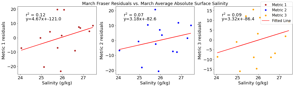
[78]:
# ---------- Halocline ---------
fig4,ax4=plt.subplots(1,3,figsize=(17,5),constrained_layout=True)
ax4[0].plot(halomar,fraserresid1,'o',color='firebrick',label='Metric 1')
ax4[0].set_xlabel('Halocline Depth (m)')
ax4[0].set_ylabel('Metric 1 residuals')
y,r2,m,b=bloomdrivers.reg_r2(halomar,fraserresid1)
ax4[0].plot(halomar, y, 'r')
ax4[0].text(0.1, 0.85, '$\mathregular{r^2}$ = %.2f'%r2, transform=ax4[0].transAxes)
ax4[0].text(0.1,0.78,f'y={round(m,2)}x+{round(b,1)}',horizontalalignment='left',verticalalignment='bottom',transform=ax4[0].transAxes)

ax4[1].plot(halomar,fraserresid2,'o',color='b',label='Metric 2')
ax4[1].set_xlabel('Halocline Depth (m)')
ax4[1].set_ylabel('Metric 2 residuals')
ax4[1].set_title('March Salinity Residuals vs. March Halocline Depth')
y,r2,m,b=bloomdrivers.reg_r2(halomar,fraserresid2)
ax4[1].plot(halomar, y, 'r')
ax4[1].text(0.1, 0.85, '$\mathregular{r^2}$ = %.2f'%r2, transform=ax4[1].transAxes)
ax4[1].text(0.1,0.78,f'y={round(m,2)}x+{round(b,1)}',horizontalalignment='left',verticalalignment='bottom',transform=ax4[1].transAxes)

ax4[2].plot(halomar,fraserresid3,'o',color='orange',label='Metric 3')
ax4[2].set_xlabel('Halocline Depth (m)')
ax4[2].set_ylabel('Metric 3 residuals')
y,r2,m,b=bloomdrivers.reg_r2(halomar,fraserresid3)
ax4[2].plot(halomar, y, 'r', label='Fitted Line')
ax4[2].text(0.1, 0.85, '$\mathregular{r^2}$ = %.2f'%r2, transform=ax4[2].transAxes)
ax4[2].text(0.1,0.78,f'y={round(m,2)}x+{round(b,1)}',horizontalalignment='left',verticalalignment='bottom',transform=ax4[2].transAxes)
fig4.legend()
[78]:
<matplotlib.legend.Legend at 0x7f65280de7f0>
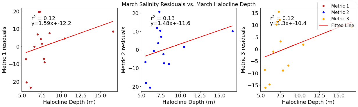
Multiple linear regression
Correlation with winds (least to greatest) * Fraser, temp, salinity, density diffs, midno3, deepno3, halocline, solar, eddy30, eddy15, turbocline
Correlation with solar * Fraser, temp, midno3, halo, sal, density diffs, deepno3, eddy30, eddy15, turbo, wind
Correlation with temperature * density diffs, salinity, halo, solar, turbo, eddy30, eddy15, wind, deepno3, midno3, fraser
Correlation with midno3 * density diffs, solar/salinity, halocline, fraser/temp, turbo/eddy30, wind/eddy15, deepno3
Correlation with deep no3 * density diffs, Fraser, salinity, halo, solar, turbo, temp, eddy30/eddy15, wind, midno3
Correlation with salinity * Temp, deepno3, midno3, solar, fraser, wind, eddy30,eddy15, turbo, halo, density diffs
Correlation with fraser * Wind, halo, deepno3, eddy30, eddy15, solar/turbo, density diffs, sal, midno3, temp
Correlation with halocline * Fraser, temp, deep no3, midno3/solar, wind, salinity, density diffs, turbo, eddy15, eddy30
[79]:
# make a table
variables=list()
rsquared=list()
adjusted_r2=list()
MLR with wind, and bloom date:
[80]:
A=np.vstack((windmar,np.ones(np.shape(windmar)))).T
b=yearday2
m=np.linalg.lstsq(A,b,rcond=None)[0]
model, resid = np.linalg.lstsq(A, b,rcond=None)[:2]
r2 = 1 - resid / (len(b) * np.var(b))
p=1 # number of parameters
ar2= 1-(len(b)-1)/(len(b)-p)*(1-r2)
print('Coefficients and intercept:')
print(m)
print('r2 value:')
print(r2)
print('adjusted r2 value:')
print(ar2)
variables.append('Wind')
rsquared.append(np.round(r2,2))
adjusted_r2.append(np.round(ar2,2))
Coefficients and intercept:
[12.17933716 31.71336845]
r2 value:
[0.61225758]
adjusted r2 value:
[0.61225758]
MLR with solar, and bloom date:
[81]:
A=np.vstack((solarmar,np.ones(np.shape(windmar)))).T
b=yearday2
m=np.linalg.lstsq(A,b,rcond=None)[0]
model, resid = np.linalg.lstsq(A, b,rcond=None)[:2]
r2 = 1 - resid / (len(b) * np.var(b))
p=1 # number of parameters
ar2= 1-(len(b)-1)/(len(b)-p)*(1-r2)
print('Coefficients and intercept:')
print(m)
print('r2 value:')
print(r2)
print('adjusted r2 value:')
print(ar2)
variables.append('Solar')
rsquared.append(np.round(r2,2))
adjusted_r2.append(np.round(ar2,2))
Coefficients and intercept:
[ -0.45009544 151.87535404]
r2 value:
[0.45001727]
adjusted r2 value:
[0.45001727]
MLR with temperature, and bloom date:
[82]:
A=np.vstack((tempmar,np.ones(np.shape(windmar)))).T
b=yearday2
m=np.linalg.lstsq(A,b,rcond=None)[0]
model, resid = np.linalg.lstsq(A, b,rcond=None)[:2]
r2 = 1 - resid / (len(b) * np.var(b))
p=1 # number of parameters
ar2= 1-(len(b)-1)/(len(b)-p)*(1-r2)
print('Coefficients and intercept:')
print(m)
print('r2 value:')
print(r2)
print('adjusted r2 value:')
print(ar2)
variables.append('Temperature')
rsquared.append(np.round(r2,2))
adjusted_r2.append(np.round(ar2,2))
Coefficients and intercept:
[-14.73236206 208.81350317]
r2 value:
[0.55382549]
adjusted r2 value:
[0.55382549]
MLR with fraser, and bloom date:
[83]:
A=np.vstack((frasermar,np.ones(np.shape(windmar)))).T
b=yearday2
m=np.linalg.lstsq(A,b,rcond=None)[0]
model, resid = np.linalg.lstsq(A, b,rcond=None)[:2]
r2 = 1 - resid / (len(b) * np.var(b))
p=1 # number of parameters
ar2= 1-(len(b)-1)/(len(b)-p)*(1-r2)
print('Coefficients and intercept:')
print(m)
print('r2 value:')
print(r2)
print('adjusted r2 value:')
print(ar2)
variables.append('Fraser')
rsquared.append(np.round(r2,2))
adjusted_r2.append(np.round(ar2,2))
Coefficients and intercept:
[-1.38639159e-02  1.12510764e+02]
r2 value:
[0.24956061]
adjusted r2 value:
[0.24956061]
MLR with wind+solar, and bloom date:
[84]:
A=np.vstack((windmar,solarmar,np.ones(np.shape(windmar)))).T
b=yearday2
m=np.linalg.lstsq(A,b,rcond=None)[0]
model, resid = np.linalg.lstsq(A, b,rcond=None)[:2]
r2 = 1 - resid / (len(b) * np.var(b))
p=2 # number of parameters
ar2= 1-(len(b)-1)/(len(b)-p)*(1-r2)
print('Coefficients and intercept:')
print(m)
print('r2 value:')
print(r2)
print('adjusted r2 value:')
print(ar2)
variables.append('Wind, Solar')
rsquared.append(np.round(r2,2))
adjusted_r2.append(np.round(ar2,2))
Coefficients and intercept:
[10.82007059 -0.07234256 47.79854457]
r2 value:
[0.61625698]
adjusted r2 value:
[0.5842784]
MLR with wind+temperature, and bloom date:
[85]:
A=np.vstack((windmar,tempmar,np.ones(np.shape(windmar)))).T
b=yearday2
m=np.linalg.lstsq(A,b,rcond=None)[0]
model, resid = np.linalg.lstsq(A, b,rcond=None)[:2]
r2 = 1 - resid / (len(b) * np.var(b))
p=2 # number of parameters
ar2= 1-(len(b)-1)/(len(b)-p)*(1-r2)
print('Coefficients and intercept:')
print(m)
print('r2 value:')
print(r2)
print('adjusted r2 value:')
print(ar2)
variables.append('Wind, Temperature')
rsquared.append(np.round(r2,2))
adjusted_r2.append(np.round(ar2,2))
Coefficients and intercept:
[  9.12509613 -10.39586926 126.79153497]
r2 value:
[0.84952643]
adjusted r2 value:
[0.83698697]
MLR with wind+fraser, and bloom date:
[86]:
A=np.vstack((windmar,frasermar,np.ones(np.shape(windmar)))).T
b=yearday2
m=np.linalg.lstsq(A,b,rcond=None)[0]
model, resid = np.linalg.lstsq(A, b,rcond=None)[:2]
r2 = 1 - resid / (len(b) * np.var(b))
p=2 # number of parameters
ar2= 1-(len(b)-1)/(len(b)-p)*(1-r2)
print('Coefficients and intercept:')
print(m)
print('r2 value:')
print(r2)
print('adjusted r2 value:')
print(ar2)
variables.append('Wind, Fraser')
rsquared.append(np.round(r2,2))
adjusted_r2.append(np.round(ar2,2))
Coefficients and intercept:
[ 1.16826411e+01 -1.23730538e-02  4.78536796e+01]
r2 value:
[0.81001257]
adjusted r2 value:
[0.79418029]
MLR with solar+temperature, and bloom date:
[87]:
A=np.vstack((solarmar,tempmar,np.ones(np.shape(solarmar)))).T
b=yearday2
m=np.linalg.lstsq(A,b,rcond=None)[0]
model, resid = np.linalg.lstsq(A, b,rcond=None)[:2]
r2 = 1 - resid / (len(b) * np.var(b))
p=2 # number of parameters
ar2= 1-(len(b)-1)/(len(b)-p)*(1-r2)
print('Coefficients and intercept:')
print(m)
print('r2 value:')
print(r2)
print('adjusted r2 value:')
print(ar2)
variables.append('Solar, Temperature')
rsquared.append(np.round(r2,2))
adjusted_r2.append(np.round(ar2,2))
Coefficients and intercept:
[ -0.36257936 -12.52727288 236.00199884]
r2 value:
[0.8334472]
adjusted r2 value:
[0.8195678]
MLR with solar+fraser, and bloom date:
[88]:
A=np.vstack((solarmar,frasermar,np.ones(np.shape(frasermar)))).T
b=yearday2
m=np.linalg.lstsq(A,b,rcond=None)[0]
model, resid = np.linalg.lstsq(A, b,rcond=None)[:2]
r2 = 1 - resid / (len(b) * np.var(b))
p=2 # number of parameters
ar2= 1-(len(b)-1)/(len(b)-p)*(1-r2)
print('Coefficients and intercept:')
print(m)
print('r2 value:')
print(r2)
print('adjusted r2 value:')
print(ar2)
variables.append('Solar, Fraser')
rsquared.append(np.round(r2,2))
adjusted_r2.append(np.round(ar2,2))
Coefficients and intercept:
[-5.26209771e-01 -1.77289847e-02  1.80369592e+02]
r2 value:
[0.84525305]
adjusted r2 value:
[0.83235747]
MLR with fraser+temperature, and bloom date:
[89]:
A=np.vstack((frasermar,tempmar,np.ones(np.shape(tempmar)))).T
b=yearday2
m=np.linalg.lstsq(A,b,rcond=None)[0]
model, resid = np.linalg.lstsq(A, b,rcond=None)[:2]
r2 = 1 - resid / (len(b) * np.var(b))
p=2 # number of parameters
ar2= 1-(len(b)-1)/(len(b)-p)*(1-r2)
print('Coefficients and intercept:')
print(m)
print('r2 value:')
print(r2)
print('adjusted r2 value:')
print(ar2)
variables.append('Fraser, Temperature')
rsquared.append(np.round(r2,2))
adjusted_r2.append(np.round(ar2,2))
Coefficients and intercept:
[ 2.40916158e-03 -1.59806565e+01  2.15630446e+02]
r2 value:
[0.55738527]
adjusted r2 value:
[0.5205007]
MLR with solar+wind+temperature, and bloom date:
[90]:
A=np.vstack((solarmar,windmar,tempmar,np.ones(np.shape(solarmar)))).T
b=yearday2
m=np.linalg.lstsq(A,b,rcond=None)[0]
model, resid = np.linalg.lstsq(A, b,rcond=None)[:2]
r2 = 1 - resid / (len(b) * np.var(b))
p=3 # number of parameters
ar2= 1-(len(b)-1)/(len(b)-p)*(1-r2)
print('Coefficients and intercept:')
print(m)
print('r2 value:')
print(r2)
print('adjusted r2 value:')
print(ar2)
variables.append('Solar, Wind, Temperature')
rsquared.append(np.round(r2,2))
adjusted_r2.append(np.round(ar2,2))
Coefficients and intercept:
[ -0.17674767   5.63227106 -10.98083275 171.44085103]
r2 value:
[0.87264864]
adjusted r2 value:
[0.84949385]
MLR with wind+temperature+fraser, and bloom date:
[91]:
A=np.vstack((windmar,tempmar,frasermar,np.ones(np.shape(windmar)))).T
b=yearday2
m=np.linalg.lstsq(A,b,rcond=None)[0]
model, resid = np.linalg.lstsq(A, b,rcond=None)[:2]
r2 = 1 - resid / (len(b) * np.var(b))
p=3 # number of parameters
ar2= 1-(len(b)-1)/(len(b)-p)*(1-r2)
print('Coefficients and intercept:')
print(m)
print('r2 value:')
print(r2)
print('adjusted r2 value:')
print(ar2)
variables.append('Wind, Temperature, Fraser')
rsquared.append(np.round(r2,2))
adjusted_r2.append(np.round(ar2,2))
Coefficients and intercept:
[ 9.77142951e+00 -7.51799971e+00 -4.96138277e-03  1.06943208e+02]
r2 value:
[0.8631401]
adjusted r2 value:
[0.83825648]
MLR with solar+wind+fraser, and bloom date:
[92]:
A=np.vstack((solarmar,windmar,frasermar,np.ones(np.shape(solarmar)))).T
b=yearday2
m=np.linalg.lstsq(A,b,rcond=None)[0]
model, resid = np.linalg.lstsq(A, b,rcond=None)[:2]
r2 = 1 - resid / (len(b) * np.var(b))
p=3 # number of parameters
ar2= 1-(len(b)-1)/(len(b)-p)*(1-r2)
print('Coefficients and intercept:')
print(m)
print('r2 value:')
print(r2)
print('adjusted r2 value:')
print(ar2)
variables.append('Solar, Wind, Fraser')
rsquared.append(np.round(r2,2))
adjusted_r2.append(np.round(ar2,2))
Coefficients and intercept:
[-3.30778570e-01  5.33750305e+00 -1.56123838e-02  1.25627038e+02]
r2 value:
[0.88007271]
adjusted r2 value:
[0.85826775]
MLR with solar+fraser+temperature, and bloom date:
[93]:
A=np.vstack((solarmar,frasermar,tempmar,np.ones(np.shape(solarmar)))).T
b=yearday2
m=np.linalg.lstsq(A,b,rcond=None)[0]
model, resid = np.linalg.lstsq(A, b,rcond=None)[:2]
r2 = 1 - resid / (len(b) * np.var(b))
p=3 # number of parameters
ar2= 1-(len(b)-1)/(len(b)-p)*(1-r2)
print('Coefficients and intercept:')
print(m)
print('r2 value:')
print(r2)
print('adjusted r2 value:')
print(ar2)
variables.append('Solar, Fraser, Temperature')
rsquared.append(np.round(r2,2))
adjusted_r2.append(np.round(ar2,2))
Coefficients and intercept:
[-4.49018144e-01 -1.04595361e-02 -6.58202677e+00  2.12887513e+02]
r2 value:
[0.88465392]
adjusted r2 value:
[0.8636819]
MLR with density differences+temperature, and bloom date:
[94]:
A=np.vstack((densdiff10mar,tempmar,np.ones(np.shape(densdiff10mar)))).T
b=yearday2
m=np.linalg.lstsq(A,b,rcond=None)[0]
model, resid = np.linalg.lstsq(A, b,rcond=None)[:2]
r2 = 1 - resid / (len(b) * np.var(b))
p=2 # number of parameters
ar2= 1-(len(b)-1)/(len(b)-p)*(1-r2)
print('Coefficients and intercept:')
print(m)
print('r2 value:')
print(r2)
print('adjusted r2 value:')
print(ar2)
Coefficients and intercept:
[ -6.92566003 -14.36352797 218.61282355]
r2 value:
[0.71201781]
adjusted r2 value:
[0.68801929]
MLR with midno3+solar, and bloom date:
[95]:
A=np.vstack((solarmar,midno3mar,np.ones(np.shape(solarmar)))).T
b=yearday2
m=np.linalg.lstsq(A,b,rcond=None)[0]
model, resid = np.linalg.lstsq(A, b,rcond=None)[:2]
r2 = 1 - resid / (len(b) * np.var(b))
p=2 # number of parameters
ar2= 1-(len(b)-1)/(len(b)-p)*(1-r2)
print('Coefficients and intercept:')
print(m)
print('r2 value:')
print(r2)
print('adjusted r2 value:')
print(ar2)
Coefficients and intercept:
[ -0.34499513   7.89564017 -66.14880572]
r2 value:
[0.65803171]
adjusted r2 value:
[0.62953435]
MLR with midno3+wind, and bloom date:
[96]:
A=np.vstack((windmar,midno3mar,np.ones(np.shape(solarmar)))).T
b=yearday2
m=np.linalg.lstsq(A,b,rcond=None)[0]
model, resid = np.linalg.lstsq(A, b,rcond=None)[:2]
r2 = 1 - resid / (len(b) * np.var(b))
p=2 # number of parameters
ar2= 1-(len(b)-1)/(len(b)-p)*(1-r2)
print('Coefficients and intercept:')
print(m)
print('r2 value:')
print(r2)
print('adjusted r2 value:')
print(ar2)
Coefficients and intercept:
[  9.56894808   4.53248956 -72.06034248]
r2 value:
[0.66076576]
adjusted r2 value:
[0.63249624]
MLR with midno3+solar+wind, and bloom date:
[97]:
A=np.vstack((solarmar,windmar,midno3mar,np.ones(np.shape(solarmar)))).T
b=yearday2
m=np.linalg.lstsq(A,b,rcond=None)[0]
model, resid = np.linalg.lstsq(A, b,rcond=None)[:2]
r2 = 1 - resid / (len(b) * np.var(b))
p=3 # number of parameters
ar2= 1-(len(b)-1)/(len(b)-p)*(1-r2)
print('Coefficients and intercept:')
print(m)
print('r2 value:')
print(r2)
print('adjusted r2 value:')
print(ar2)
Coefficients and intercept:
[ -0.18527469   5.40558107   5.71698379 -57.98461734]
r2 value:
[0.68368538]
adjusted r2 value:
[0.62617363]
[98]:
mlr_df=pd.DataFrame({'Environmental Drivers':variables,'R-squared':rsquared,'Adjusted R-squared':adjusted_r2})
mlr_df.sort_values(by=['Adjusted R-squared'],ascending=False,inplace=True)
mlr_df
[98]:
| Environmental Drivers | R-squared | Adjusted R-squared | |
|---|---|---|---|
| 12 | Solar, Wind, Fraser | [0.88] | [0.86] |
| 13 | Solar, Fraser, Temperature | [0.88] | [0.86] |
| 10 | Solar, Wind, Temperature | [0.87] | [0.85] |
| 5 | Wind, Temperature | [0.85] | [0.84] |
| 11 | Wind, Temperature, Fraser | [0.86] | [0.84] |
| 8 | Solar, Fraser | [0.85] | [0.83] |
| 7 | Solar, Temperature | [0.83] | [0.82] |
| 6 | Wind, Fraser | [0.81] | [0.79] |
| 0 | Wind | [0.61] | [0.61] |
| 4 | Wind, Solar | [0.62] | [0.58] |
| 2 | Temperature | [0.55] | [0.55] |
| 9 | Fraser, Temperature | [0.56] | [0.52] |
| 1 | Solar | [0.45] | [0.45] |
| 3 | Fraser | [0.25] | [0.25] |
[ ]:
Conclusions
Metric 1 was not as consistent as Metrics 2 and 3, so it was not heavily weighted. Only March values were considered, as they showed the highest correlations across all environmental drivers.
Primary driver: Wind speed cubed * average correlation coefficient of metrics 2&3: 0.785
Secondar driver: Solar radiation: * average correlation coefficient of metrics 2&3: 0.69
Tertiary driver: Surface temperature: * average correlation coefficient of metrics 2&3: 0.655
Tertiary driver: Fraser flow: * average correlation coefficient of the metrics 2&3: 0.435 * weak correlation with bloom timing, but had the highest correlation with both wind residuals and solar residuals