Time Series of Phytoplankton Bloom Timing and Environmental Drivers from 2007-2020 at Station QU39 (201905 model run)
To run this notebook, pickle files for each year of interest must be created in the ‘makePickles201905’ notebook.
[1]:
import numpy as np
import matplotlib.pyplot as plt
import matplotlib.dates as mdates
import matplotlib as mpl
import netCDF4 as nc
import datetime as dt
from salishsea_tools import evaltools as et, places, viz_tools, visualisations, bloomdrivers
import xarray as xr
import pandas as pd
import pickle
import os

%matplotlib inline
To recreate this notebook at a different location
follow these instructions: Change only the values in the following cell. If you change the startyear and endyear, the xticks (years) in the plots will need to be adjusted accordingly. If you did not make pickle files for 201812 bloom timing variables, remove the cell that loads that data ‘Load bloom timing variables for 201812 run’, as well as a section from the cell that plots bloom timing; ‘Bloom Date’. The code to create 201812 pickles files can be found at
/ocean/aisabell/MEOPAR/Analysis-Aline/notebooks/Bloom_Timing/stationS3/201812EnvironmentalDrivers.ipynb.
[2]:
# The path to the directory where the pickle files are stored:
savedir='/ocean/aisabell/MEOPAR/extracted_files'

# Change 'S3' to the location of interest
loc='QU39'
# Note: x and y limits in the following cell (map of location) may need to be adjusted

# What is the start year and end year+1 of the time range of interest?
startyear=2007
endyear=2021 # does NOT include this value

# Note: pickle file with 'non-location specific variables' only need to be created for each year, not for each location
# Note: xticks (years) in the plots will need to be changed
# Note: 201812 bloom timing variable load and plotting will also need to be removed
[3]:
modver='201905'
# lat and lon information for place:
lon,lat=places.PLACES[loc]['lon lat']
# get place information on SalishSeaCast grid:
ij,ii=places.PLACES[loc]['NEMO grid ji']
jw,iw=places.PLACES[loc]['GEM2.5 grid ji']
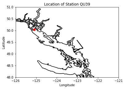
fig, ax = plt.subplots(1,1,figsize = (6,6))
with xr.open_dataset('/data/vdo/MEOPAR/NEMO-forcing/grid/mesh_mask201702.nc') as mesh:
ax.contour(mesh.nav_lon,mesh.nav_lat,mesh.tmask.isel(t=0,z=0),[0.1,],colors='k')
tmask=np.array(mesh.tmask)
gdept_1d=np.array(mesh.gdept_1d)
e3t_0=np.array(mesh.e3t_0)
ax.plot(lon, lat, '.', markersize=14, color='red')
ax.set_ylim(48,51)
ax.set_xlim(-126,-121)
ax.set_title('Location of Station %s'%loc)
ax.set_xlabel('Longitude')
ax.set_ylabel('Latitude')
viz_tools.set_aspect(ax,coords='map')
[3]:
1.1363636363636362
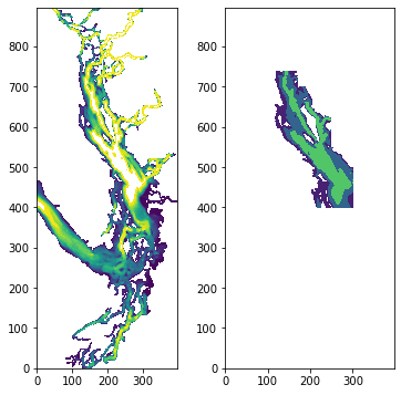
Strait of Georgia Region
[4]:
# define sog region:
fig, ax = plt.subplots(1,2,figsize = (6,6))
with xr.open_dataset('/data/vdo/MEOPAR/NEMO-forcing/grid/bathymetry_201702.nc') as bathy:
    bath=np.array(bathy.Bathymetry)
ax[0].contourf(bath,np.arange(0,250,10))
viz_tools.set_aspect(ax[0],coords='grid')
sogmask=np.copy(tmask[:,:,:,:])
sogmask[:,:,740:,:]=0
sogmask[:,:,700:,170:]=0
sogmask[:,:,550:,250:]=0
sogmask[:,:,:,302:]=0
sogmask[:,:,:400,:]=0
sogmask[:,:,:,:100]=0
#sogmask250[bath<250]=0
ax[1].contourf(np.ma.masked_where(sogmask[0,0,:,:]==0,bathy.Bathymetry),[0,100,250,550])
[4]:
<matplotlib.contour.QuadContourSet at 0x7f710a9098e0>
** Stop and check, have you made pickle files for all the years? **
Load bloom timing variables for 201905 run
[5]:
# loop through years of spring time series (mid feb-june) for bloom timing for 201905 run
years=list()
bloomtime1=list()
bloomtime2=list()
bloomtime3=list()
for year in range(startyear,endyear):
    fname3=f'springBloomTime_{str(year)}_{loc}_{modver}.pkl'
    savepath3=os.path.join(savedir,fname3)
    bio_time0,sno30,sdiat0,sflag0,scili0,diat_alld0,no3_alld0,flag_alld0,cili_alld0,phyto_alld0,\
                 intdiat0,intphyto0,fracdiat0,sphyto0,percdiat0=pickle.load(open(savepath3,'rb'))
    # put code that calculates bloom timing here
    bt1=bloomdrivers.metric1_bloomtime(phyto_alld0,no3_alld0,bio_time0)
    bt2=bloomdrivers.metric2_bloomtime(phyto_alld0,no3_alld0,bio_time0)
    bt3=bloomdrivers.metric3_bloomtime(sphyto0,sno30,bio_time0)
    years.append(year)
    bloomtime1.append(bt1)
    bloomtime2.append(bt2)
    bloomtime3.append(bt3)
years=np.array(years)
bloomtime1=np.array(bloomtime1)
bloomtime2=np.array(bloomtime2)
bloomtime3=np.array(bloomtime3)

# get year day
yearday1=et.datetimeToYD(bloomtime1)  # convert to year day tool
yearday2=et.datetimeToYD(bloomtime2)
yearday3=et.datetimeToYD(bloomtime3)
Combine separate year files into arrays:
[6]:
# loop through years (for location specific drivers)

years=list()
windjan=list()
windfeb=list()
windmar=list()
solarjan=list()
solarfeb=list()
solarmar=list()
parjan=list()
parfeb=list()
parmar=list()
tempjan=list()
tempfeb=list()
tempmar=list()
saljan=list()
salfeb=list()
salmar=list()
zoojan=list()
zoofeb=list()
zoomar=list()
mesozoojan=list()
mesozoofeb=list()
mesozoomar=list()
microzoojan=list()
microzoofeb=list()
microzoomar=list()
intzoojan=list()
intzoofeb=list()
intzoomar=list()
intmesozoojan=list()
intmesozoofeb=list()
intmesozoomar=list()
intmicrozoojan=list()
intmicrozoofeb=list()
intmicrozoomar=list()
midno3jan=list()
midno3feb=list()
midno3mar=list()

for year in range(startyear,endyear):
    fname=f'JanToMarch_TimeSeries_{year}_{loc}_{modver}.pkl'
    savepath=os.path.join(savedir,fname)
    bio_time,diat_alld,no3_alld,flag_alld,cili_alld,microzoo_alld,mesozoo_alld,\
            intdiat,intphyto,spar,intmesoz,intmicroz,grid_time,temp,salinity,u_wind,v_wind,twind,\
            solar,no3_30to90m,sno3,sdiat,sflag,scili,intzoop,fracdiat,zoop_alld,sphyto,phyto_alld,\
            percdiat,wspeed,winddirec=pickle.load(open(savepath,'rb'))
    # put code that calculates drivers here
    wind=bloomdrivers.D1_3monthly_avg(twind,wspeed)
    solar=bloomdrivers.D1_3monthly_avg(twind,solar)
    par=bloomdrivers.D1_3monthly_avg(bio_time,spar)
    temp=bloomdrivers.D1_3monthly_avg(grid_time,temp)
    sal=bloomdrivers.D1_3monthly_avg(grid_time,salinity)
    zoo=bloomdrivers.D2_3monthly_avg(bio_time,zoop_alld)
    mesozoo=bloomdrivers.D2_3monthly_avg(bio_time,mesozoo_alld)
    microzoo=bloomdrivers.D2_3monthly_avg(bio_time,microzoo_alld)
    intzoo=bloomdrivers.D1_3monthly_avg(bio_time,intzoop)
    intmesozoo=bloomdrivers.D1_3monthly_avg(bio_time,intmesoz)
    intmicrozoo=bloomdrivers.D1_3monthly_avg(bio_time,intmicroz)
    midno3=bloomdrivers.D1_3monthly_avg(bio_time,no3_30to90m)

    years.append(year)
    windjan.append(wind[0])
    windfeb.append(wind[1])
    windmar.append(wind[2])
    solarjan.append(solar[0])
    solarfeb.append(solar[1])
    solarmar.append(solar[2])
    parjan.append(par[0])
    parfeb.append(par[1])
    parmar.append(par[2])
    tempjan.append(temp[0])
    tempfeb.append(temp[1])
    tempmar.append(temp[2])
    saljan.append(sal[0])
    salfeb.append(sal[1])
    salmar.append(sal[2])
    zoojan.append(zoo[0])
    zoofeb.append(zoo[1])
    zoomar.append(zoo[2])
    mesozoojan.append(mesozoo[0])
    mesozoofeb.append(mesozoo[1])
    mesozoomar.append(mesozoo[2])
    microzoojan.append(microzoo[0])
    microzoofeb.append(microzoo[1])
    microzoomar.append(microzoo[2])
    intzoojan.append(intzoo[0])
    intzoofeb.append(intzoo[1])
    intzoomar.append(intzoo[2])
    intmesozoojan.append(intmesozoo[0])
    intmesozoofeb.append(intmesozoo[1])
    intmesozoomar.append(intmesozoo[2])
    intmicrozoojan.append(intmicrozoo[0])
    intmicrozoofeb.append(intmicrozoo[1])
    intmicrozoomar.append(intmicrozoo[2])
    midno3jan.append(midno3[0])
    midno3feb.append(midno3[1])
    midno3mar.append(midno3[2])

years=np.array(years)
windjan=np.array(windjan)
windfeb=np.array(windfeb)
windmar=np.array(windmar)
solarjan=np.array(solarjan)
solarfeb=np.array(solarfeb)
solarmar=np.array(solarmar)
parjan=np.array(parjan)
parfeb=np.array(parfeb)
parmar=np.array(parmar)
tempjan=np.array(tempjan)
tempfeb=np.array(tempfeb)
tempmar=np.array(tempmar)
saljan=np.array(saljan)
salfeb=np.array(salfeb)
salmar=np.array(salmar)
zoojan=np.array(zoojan)
zoofeb=np.array(zoofeb)
zoomar=np.array(zoomar)
mesozoojan=np.array(mesozoojan)
mesozoofeb=np.array(mesozoofeb)
mesozoomar=np.array(mesozoomar)
microzoojan=np.array(microzoojan)
microzoofeb=np.array(microzoofeb)
microzoomar=np.array(microzoomar)
intzoojan=np.array(intzoojan)
intzoofeb=np.array(intzoofeb)
intzoomar=np.array(intzoomar)
intmesozoojan=np.array(intmesozoojan)
intmesozoofeb=np.array(intmesozoofeb)
intmesozoomar=np.array(intmesozoomar)
intmicrozoojan=np.array(intmicrozoojan)
intmicrozoofeb=np.array(intmicrozoofeb)
intmicrozoomar=np.array(intmicrozoomar)
midno3jan=np.array(midno3jan)
midno3feb=np.array(midno3feb)
midno3mar=np.array(midno3mar)
[7]:
# loop through years (for non-location specific drivers)
fraserjan=list()
fraserfeb=list()
frasermar=list()
deepno3jan=list()
deepno3feb=list()
deepno3mar=list()

for year in range(startyear,endyear):
    fname2=f'JanToMarch_TimeSeries_{year}_{modver}.pkl'
    savepath2=os.path.join(savedir,fname2)
    no3_past250m,riv_time,rivFlow=pickle.load(open(savepath2,'rb'))
    # Code that calculates drivers here
    fraser=bloomdrivers.D1_3monthly_avg2(riv_time,rivFlow)
    fraserjan.append(fraser[0])
    fraserfeb.append(fraser[1])
    frasermar.append(fraser[2])

    fname=f'JanToMarch_TimeSeries_{year}_{loc}_{modver}.pkl'
    savepath=os.path.join(savedir,fname)
    bio_time,diat_alld,no3_alld,flag_alld,cili_alld,microzoo_alld,mesozoo_alld,\
            intdiat,intphyto,spar,intmesoz,intmicroz,grid_time,temp,salinity,u_wind,v_wind,twind,\
            solar,no3_30to90m,sno3,sdiat,sflag,scili,intzoop,fracdiat,zoop_alld,sphyto,phyto_alld,\
            percdiat,wspeed,winddirec=pickle.load(open(savepath,'rb'))
    deepno3=bloomdrivers.D1_3monthly_avg(bio_time,no3_past250m)

    deepno3jan.append(deepno3[0])
    deepno3feb.append(deepno3[1])
    deepno3mar.append(deepno3[2])

fraserjan=np.array(fraserjan)
fraserfeb=np.array(fraserfeb)
frasermar=np.array(frasermar)
deepno3jan=np.array(deepno3jan)
deepno3feb=np.array(deepno3feb)
deepno3mar=np.array(deepno3mar)
[8]:
# for T grid depth:
startd=dt.datetime(2015,1,1) # some date to get depth
endd=dt.datetime(2015,1,2)
basedir='/results2/SalishSea/nowcast-green.201905/'
nam_fmt='nowcast'
flen=1 # files contain 1 day of data each
tres=24 # 1: hourly resolution; 24: daily resolution
flist=et.index_model_files(startd,endd,basedir,nam_fmt,flen,"grid_T",tres)
with xr.open_mfdataset(flist['paths']) as gridt:
    depth_T=np.array(gridt.deptht)

# loop through years (for mixing drivers)

halojan=list()
halofeb=list()
halomar=list()
turbojan=list()
turbofeb=list()
turbomar=list()
densdiff5jan=list()
densdiff10jan=list()
densdiff15jan=list()
densdiff20jan=list()
densdiff25jan=list()
densdiff30jan=list()
densdiff5feb=list()
densdiff10feb=list()
densdiff15feb=list()
densdiff20feb=list()
densdiff25feb=list()
densdiff30feb=list()
densdiff5mar=list()
densdiff10mar=list()
densdiff15mar=list()
densdiff20mar=list()
densdiff25mar=list()
densdiff30mar=list()
eddy15jan=list()
eddy15feb=list()
eddy15mar=list()
eddy30jan=list()
eddy30feb=list()
eddy30mar=list()

for year in range(startyear,endyear):
    fname4=f'JanToMarch_Mixing_{year}_{loc}_{modver}.pkl'
    savepath4=os.path.join(savedir,fname4)
    halocline,eddy,depth,grid_time,temp,salinity=pickle.load(open(savepath4,'rb'))

    # halocline
    halo=bloomdrivers.D1_3monthly_avg(grid_time,halocline)
    halojan.append(halo[0])
    halofeb.append(halo[1])
    halomar.append(halo[2])
    # turbocline
    turbo=bloomdrivers.turbo(eddy,grid_time,depth_T)
    turbojan.append(turbo[0])
    turbofeb.append(turbo[1])
    turbomar.append(turbo[2])
    # density differences
    dict_diffs=bloomdrivers.density_diff(salinity,temp,grid_time)
    values=dict_diffs.values()
    all_diffs=list(values)
    densdiff5jan.append(all_diffs[0])
    densdiff10jan.append(all_diffs[3])
    densdiff15jan.append(all_diffs[6])
    densdiff20jan.append(all_diffs[9])
    densdiff25jan.append(all_diffs[12])
    densdiff30jan.append(all_diffs[15])
    densdiff5feb.append(all_diffs[1])
    densdiff10feb.append(all_diffs[4])
    densdiff15feb.append(all_diffs[7])
    densdiff20feb.append(all_diffs[10])
    densdiff25feb.append(all_diffs[13])
    densdiff30feb.append(all_diffs[16])
    densdiff5mar.append(all_diffs[2])
    densdiff10mar.append(all_diffs[5])
    densdiff15mar.append(all_diffs[8])
    densdiff20mar.append(all_diffs[11])
    densdiff25mar.append(all_diffs[14])
    densdiff30mar.append(all_diffs[17])
    # average eddy diffusivity
    avg_eddy=bloomdrivers.avg_eddy(eddy,grid_time,ij,ii)
    eddy15jan.append(avg_eddy[0])
    eddy15feb.append(avg_eddy[1])
    eddy15mar.append(avg_eddy[2])
    eddy30jan.append(avg_eddy[3])
    eddy30feb.append(avg_eddy[4])
    eddy30mar.append(avg_eddy[5])

halojan=np.array(halojan)
halofeb=np.array(halofeb)
halomar=np.array(halomar)
turbojan=np.array(turbojan)
turbofeb=np.array(turbofeb)
turbomar=np.array(turbomar)
densdiff5jan=np.array(densdiff5jan)
densdiff10jan=np.array(densdiff10jan)
densdiff15jan=np.array(densdiff15jan)
densdiff20jan=np.array(densdiff20jan)
densdiff25jan=np.array(densdiff25jan)
densdiff30jan=np.array(densdiff30jan)
densdiff5feb=np.array(densdiff5feb)
densdiff10feb=np.array(densdiff10feb)
densdiff15feb=np.array(densdiff15feb)
densdiff20feb=np.array(densdiff20feb)
densdiff25feb=np.array(densdiff25feb)
densdiff30feb=np.array(densdiff30feb)
densdiff5mar=np.array(densdiff5mar)
densdiff10mar=np.array(densdiff10mar)
densdiff15mar=np.array(densdiff15mar)
densdiff20mar=np.array(densdiff20mar)
densdiff25mar=np.array(densdiff25mar)
densdiff30mar=np.array(densdiff30mar)
eddy15jan=np.array(eddy15jan)
eddy15feb=np.array(eddy15feb)
eddy15mar=np.array(eddy15mar)
eddy30jan=np.array(eddy30jan)
eddy30feb=np.array(eddy30feb)
eddy30mar=np.array(eddy30mar)
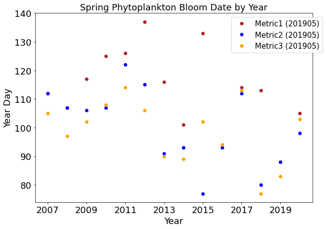
Bloom Date Time Series
[9]:
SMALL_SIZE = 15
MEDIUM_SIZE = 18
BIGGER_SIZE = 21

plt.rc('font', size=MEDIUM_SIZE)          # controls default text sizes
plt.rc('axes', titlesize=MEDIUM_SIZE)     # fontsize of the axes title
plt.rc('axes', labelsize=MEDIUM_SIZE)    # fontsize of the x and y labels
plt.rc('xtick', labelsize=MEDIUM_SIZE)    # fontsize of the tick labels
plt.rc('ytick', labelsize=MEDIUM_SIZE)    # fontsize of the tick labels
plt.rc('legend', fontsize=SMALL_SIZE)    # legend fontsize
plt.rc('figure', titlesize=BIGGER_SIZE)  # fontsize of the figure title
[10]:
# plot bloomtime for each year:
fig,ax=plt.subplots(1,1,figsize=(10,7))
p1=ax.plot(years,yearday1, 'o',color='firebrick',label='Metric1 (201905)')
p2=ax.plot(years,yearday2, 'o',color='b',label='Metric2 (201905)')
p3=ax.plot(years,yearday3, 'o',color='orange',label='Metric3 (201905)')
ax.set_ylabel('Year Day')
ax.set_xlabel('Year')
ax.set_title('Spring Phytoplankton Bloom Date by Year')
ax.set_xticks([2007,2009,2011,2013,2015,2017,2019])
ax.legend(handles=[p1[0],p2[0],p3[0]],bbox_to_anchor=(1.05, 1.0))
[10]:
<matplotlib.legend.Legend at 0x7f710a089430>
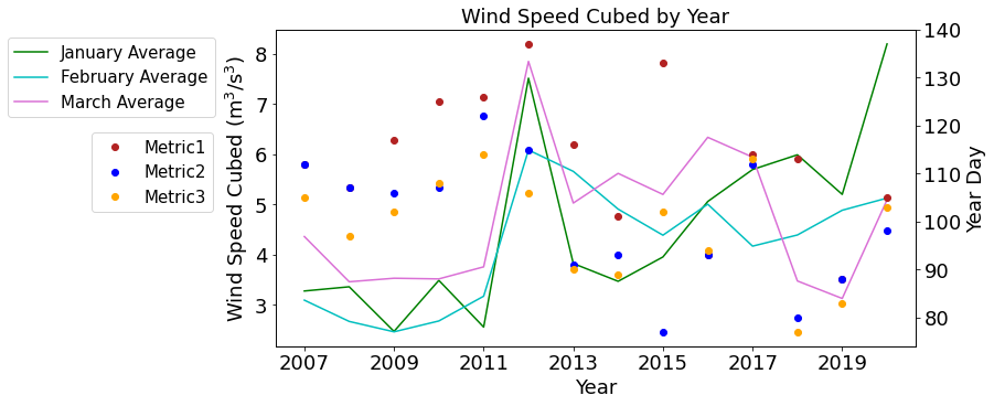
Monthly average wind speed cubed (January-March)
[11]:
fig,ax=plt.subplots(1,1,figsize=(12,5),constrained_layout=True)
p1=ax.plot(years,windjan, '-',color='green',label='January Average')
p2=ax.plot(years,windfeb, '-',color='c',label='February Average')
p3=ax.plot(years,windmar, '-',color='orchid',label='March Average')
ax.set_ylabel('Wind Speed Cubed ($\mathregular{m^3}$/$\mathregular{s^3}$)')
ax.set_xlabel('Year')
ax.set_title('Wind Speed Cubed by Year')
ax.set_xticks([2007,2009,2011,2013,2015,2017,2019])
ax.legend(handles=[p1[0],p2[0],p3[0]],bbox_to_anchor=(-0.43, 1.0), loc='upper left')
ax1=ax.twinx()
p4=ax1.plot(years,yearday1, 'o',color='firebrick',label='Metric1')
p5=ax1.plot(years,yearday2, 'o',color='b',label='Metric2')
p6=ax1.plot(years,yearday3, 'o',color='orange',label='Metric3')
ax1.set_ylabel('Year Day')
ax1.legend(handles=[p4[0],p5[0],p6[0]],bbox_to_anchor=(-0.3, 0.7), loc='upper left')
# ---------- Jan ---------
fig2,ax2=plt.subplots(1,3,figsize=(17,5),constrained_layout=True)
ax2[0].plot(windjan,yearday1,'o',color='firebrick')
ax2[0].set_xlabel('Wind Speed Cubed ($\mathregular{m^3}$/$\mathregular{s^3}$)')
ax2[0].set_ylabel('Bloom Day (Metric 1)')
y,r2,m,b=bloomdrivers.reg_r2(windjan,yearday1)
ax2[0].plot(windjan, y, 'r', label='Fitted Line')
ax2[0].text(0.02, 0.9, '$\mathregular{r^2}$ = %.2f'%r2,transform=ax.transAxes)
ax2[0].text(0.02,0.83,f'y={round(m,1)}x+{round(b,1)}',horizontalalignment='left',verticalalignment='bottom',transform=ax.transAxes)
ax2[1].plot(windjan,yearday2,'o',color='b')
ax2[1].set_xlabel('Wind Speed Cubed ($\mathregular{m^3}$/$\mathregular{s^3}$)')
ax2[1].set_ylabel('Bloom Day (Metric 2)')
y,r2,m,b=bloomdrivers.reg_r2(windjan,yearday2)
ax2[1].plot(windjan, y, 'r', label='Fitted line')
ax2[1].text(0.65, 0.87, '$\mathregular{r^2}$ = %.2f'%r2,transform=ax.transAxes)
ax2[1].text(0.65,0.8,f'y={round(m,1)}x+{round(b,1)}',horizontalalignment='left',verticalalignment='bottom',transform=ax.transAxes)
ax2[2].plot(windjan,yearday3,'o',color='orange')
ax2[2].set_xlabel('Wind Speed Cubed ($\mathregular{m^3}$/$\mathregular{s^3}$)')
ax2[2].set_ylabel('Bloom Day (Metric 3)')
y,r2,m,b=bloomdrivers.reg_r2(windjan,yearday3)
ax2[2].plot(windjan, y, 'r', label='Fitted line')
ax2[2].text(1.26, 0.87, '$\mathregular{r^2}$ = %.2f'%r2,transform=ax.transAxes)
ax2[2].text(1.26,0.8,f'y={round(m,1)}x+{round(b,1)}',horizontalalignment='left',verticalalignment='bottom',transform=ax.transAxes)
ax2[1].set_title('Bloom Date vs. January Average Wind Speed Cubed')
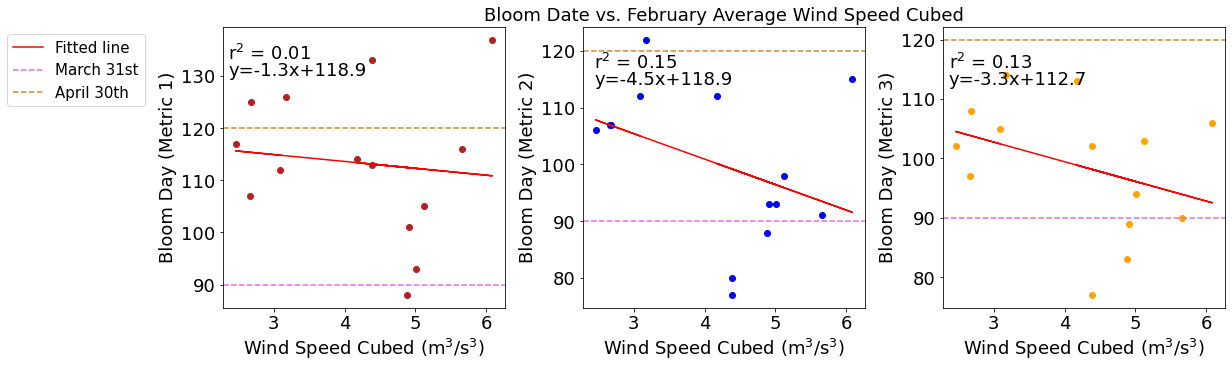
# ---------- Feb ---------
fig3,ax3=plt.subplots(1,3,figsize=(17,5),constrained_layout=True)
ax3[0].plot(windfeb,yearday1,'o',color='firebrick')
ax3[0].set_xlabel('Wind Speed Cubed ($\mathregular{m^3}$/$\mathregular{s^3}$)')
ax3[0].set_ylabel('Bloom Day (Metric 1)')
y,r2,m,b=bloomdrivers.reg_r2(windfeb,yearday1)
ax3[0].plot(windfeb, y, 'r', label='Fitted line')
ax3[0].text(0.02, 0.9, '$\mathregular{r^2}$ = %.2f'%r2,transform=ax.transAxes)
ax3[0].text(0.02,0.83,f'y={round(m,1)}x+{round(b,1)}',horizontalalignment='left',verticalalignment='bottom',transform=ax.transAxes)
ax3[1].plot(windfeb,yearday2,'o',color='b')
ax3[1].set_xlabel('Wind Speed Cubed ($\mathregular{m^3}$/$\mathregular{s^3}$)')
ax3[1].set_ylabel('Bloom Day (Metric 2)')
y,r2,m,b=bloomdrivers.reg_r2(windfeb,yearday2)
ax3[1].plot(windfeb, y, 'r', label='Fitted line')
ax3[1].text(0.65, 0.87, '$\mathregular{r^2}$ = %.2f'%r2,transform=ax.transAxes)
ax3[1].text(0.65,0.8,f'y={round(m,1)}x+{round(b,1)}',horizontalalignment='left',verticalalignment='bottom',transform=ax.transAxes)
ax3[2].plot(windfeb,yearday3,'o',color='orange')
ax3[2].set_xlabel('Wind Speed Cubed ($\mathregular{m^3}$/$\mathregular{s^3}$)')
ax3[2].set_ylabel('Bloom Day (Metric 3)')
y,r2,m,b=bloomdrivers.reg_r2(windfeb,yearday3)
ax3[2].plot(windfeb, y, 'r', label='Fitted line')
ax3[2].text(1.26, 0.87, '$\mathregular{r^2}$ = %.2f'%r2,transform=ax.transAxes)
ax3[2].text(1.26,0.8,f'y={round(m,1)}x+{round(b,1)}',horizontalalignment='left',verticalalignment='bottom',transform=ax.transAxes)
ax3[1].set_title('Bloom Date vs. February Average Wind Speed Cubed')
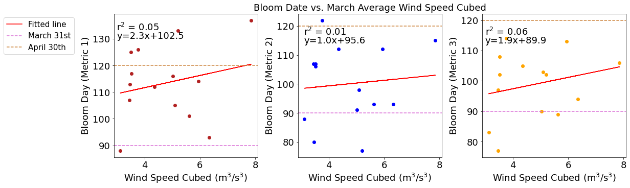
# ---------- March ---------
fig4,ax4=plt.subplots(1,3,figsize=(17,5),constrained_layout=True)
ax4[0].plot(windmar,yearday1,'o',color='firebrick')
ax4[0].set_xlabel('Wind Speed Cubed ($\mathregular{m^3}$/$\mathregular{s^3}$)')
ax4[0].set_ylabel('Bloom Day (Metric 1)')
y,r2,m,b=bloomdrivers.reg_r2(windmar,yearday1)
ax4[0].plot(windmar, y, 'r', label='Fitted line')
ax4[0].text(0.02, 0.9, '$\mathregular{r^2}$ = %.2f'%r2, transform=ax.transAxes)
ax4[0].text(0.02,0.83,f'y={round(m,1)}x+{round(b,1)}',horizontalalignment='left',verticalalignment='bottom',transform=ax.transAxes)
ax4[1].plot(windmar,yearday2,'o',color='b')
ax4[1].set_xlabel('Wind Speed Cubed ($\mathregular{m^3}$/$\mathregular{s^3}$)')
ax4[1].set_ylabel('Bloom Day (Metric 2)')
ax4[1].set_title('Bloom Date vs. March Average Wind Speed Cubed')
y,r2,m,b=bloomdrivers.reg_r2(windmar,yearday2)
ax4[1].plot(windmar, y, 'r', label='Fitted line')
ax4[1].text(0.65, 0.87, '$\mathregular{r^2}$ = %.2f'%r2, transform=ax.transAxes)
ax4[1].text(0.65,0.8,f'y={round(m,1)}x+{round(b,1)}',horizontalalignment='left',verticalalignment='bottom',transform=ax.transAxes)
ax4[2].plot(windmar,yearday3,'o',color='orange')
ax4[2].set_xlabel('Wind Speed Cubed ($\mathregular{m^3}$/$\mathregular{s^3}$)')
ax4[2].set_ylabel('Bloom Day (Metric 3)')
y,r2,m,b=bloomdrivers.reg_r2(windmar,yearday3)
ax4[2].plot(windmar, y, 'r', label='Fitted line')
ax4[2].text(1.26, 0.87, '$\mathregular{r^2}$ = %.2f'%r2, transform=ax.transAxes)
ax4[2].text(1.26,0.8,f'y={round(m,1)}x+{round(b,1)}',horizontalalignment='left',verticalalignment='bottom',transform=ax.transAxes)
# Jan month lines
ax2[0].axhline(y=90, color='orchid', linestyle='--',label='March 31st')
ax2[0].axhline(y=120, color='peru', linestyle='--',label='April 30th')
ax2[0].legend(bbox_to_anchor=(-0.25, 1.0))
ax2[1].axhline(y=90, color='orchid', linestyle='--')
ax2[2].axhline(y=90, color='orchid', linestyle='--',label='March 31st')
ax2[1].axhline(y=120, color='peru', linestyle='--')
ax2[2].axhline(y=120, color='peru', linestyle='--',label='April 30th')
# Feb month lines
ax3[0].axhline(y=90, color='orchid', linestyle='--',label='March 31st')
ax3[0].axhline(y=120, color='peru', linestyle='--',label='April 30th')
ax3[0].legend(bbox_to_anchor=(-0.25, 1.0))
ax3[1].axhline(y=90, color='orchid', linestyle='--')
ax3[2].axhline(y=90, color='orchid', linestyle='--',label='March 31st')
ax3[1].axhline(y=120, color='peru', linestyle='--')
ax3[2].axhline(y=120, color='peru', linestyle='--',label='April 30th')
# March month lines
ax4[0].axhline(y=90, color='orchid', linestyle='--',label='March 31st')
ax4[0].axhline(y=120, color='peru', linestyle='--',label='April 30th')
ax4[0].legend(bbox_to_anchor=(-0.25, 1.0))
ax4[1].axhline(y=90, color='orchid', linestyle='--')
ax4[2].axhline(y=90, color='orchid', linestyle='--',label='March 31st')
ax4[1].axhline(y=120, color='peru', linestyle='--')
ax4[2].axhline(y=120, color='peru', linestyle='--',label='April 30th')
#ax4[1].legend(handles=[p4[0],p5[0],p6[0]],bbox_to_anchor=(-1.7, 0.8), loc='upper left')
[11]:
<matplotlib.lines.Line2D at 0x7f7109d032b0>

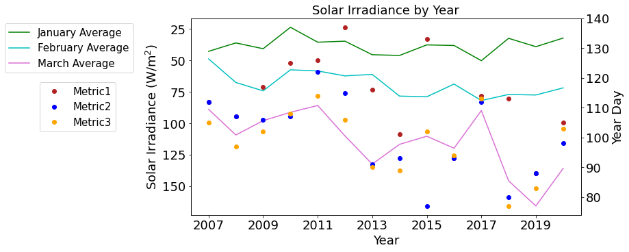
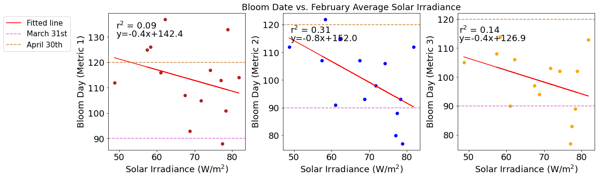
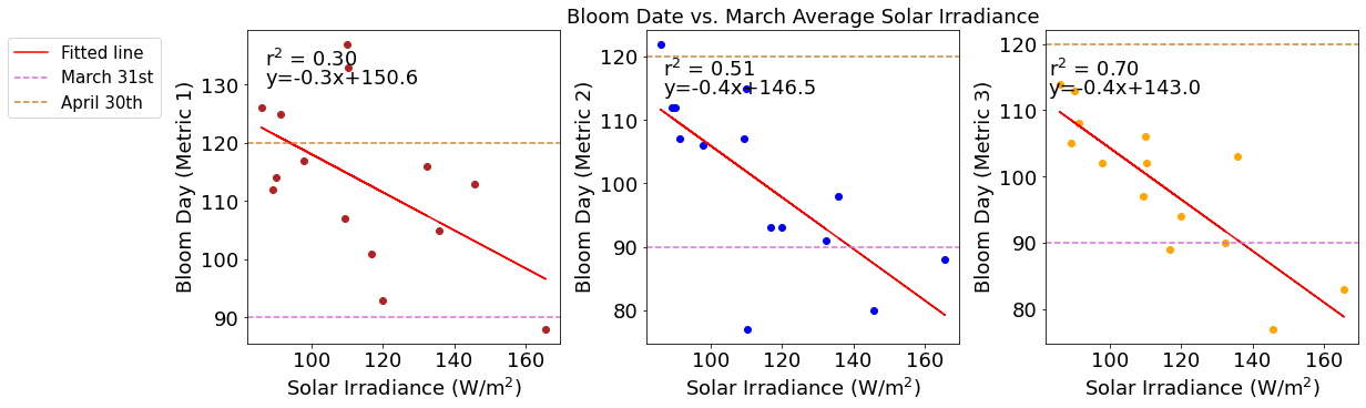
Monthly average solar radiation (January-March)
[12]:
fig,ax=plt.subplots(1,1,figsize=(12,5),constrained_layout=True)
p1=ax.plot(years,solarjan, '-',color='green',label='January Average')
p2=ax.plot(years,solarfeb, '-',color='c',label='February Average')
p3=ax.plot(years,solarmar, '-',color='orchid',label='March Average')
ax.set_ylabel('Solar Irradiance (W/$\mathregular{m^2}$)')
ax.set_xlabel('Year')
ax.set_title('Solar Irradiance by Year')
ax.set_xticks([2007,2009,2011,2013,2015,2017,2019])
ax.legend(handles=[p1[0],p2[0],p3[0]],bbox_to_anchor=(-0.49, 1.0), loc='upper left')
ax.invert_yaxis()
ax1=ax.twinx()
p4=ax1.plot(years,yearday1, 'o',color='firebrick',label='Metric1')
p5=ax1.plot(years,yearday2, 'o',color='b',label='Metric2')
p6=ax1.plot(years,yearday3, 'o',color='orange',label='Metric3')
ax1.set_ylabel('Year Day')
ax1.legend(handles=[p4[0],p5[0],p6[0]],bbox_to_anchor=(-0.4, 0.7), loc='upper left')
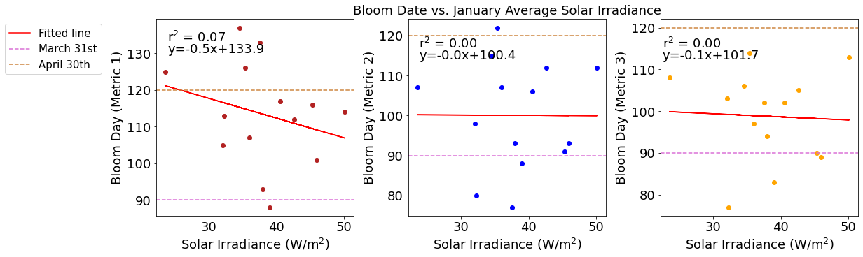
# ----Jan----
fig2,ax2=plt.subplots(1,3,figsize=(17,5),constrained_layout=True)
ax2[0].plot(solarjan,yearday1,'o',color='firebrick')
ax2[0].set_xlabel('Solar Irradiance (W/$\mathregular{m^2}$)')
ax2[0].set_ylabel('Bloom Day (Metric 1)')
y,r2,m,b=bloomdrivers.reg_r2(solarjan,yearday1)
ax2[0].plot(solarjan, y, 'r', label='Fitted line')
ax2[0].text(0.02, 0.9, '$\mathregular{r^2}$ = %.2f'%r2, transform=ax.transAxes)
ax2[0].text(0.02,0.83,f'y={round(m,1)}x+{round(b,1)}',horizontalalignment='left',verticalalignment='bottom',transform=ax.transAxes)
ax2[1].plot(solarjan,yearday2,'o',color='b')
ax2[1].set_xlabel('Solar Irradiance (W/$\mathregular{m^2}$)')
ax2[1].set_ylabel('Bloom Day (Metric 2)')
y,r2,m,b=bloomdrivers.reg_r2(solarjan,yearday2)
ax2[1].plot(solarjan, y, 'r', label='Fitted line')
ax2[1].text(0.65, 0.87, '$\mathregular{r^2}$ = %.2f'%r2, transform=ax.transAxes)
ax2[1].text(0.65,0.8,f'y={round(m,1)}x+{round(b,1)}',horizontalalignment='left',verticalalignment='bottom',transform=ax.transAxes)
ax2[2].plot(solarjan,yearday3,'o',color='orange')
ax2[2].set_xlabel('Solar Irradiance (W/$\mathregular{m^2}$)')
ax2[2].set_ylabel('Bloom Day (Metric 3)')
ax2[1].set_title('Bloom Date vs. January Average Solar Irradiance')
y,r2,m,b=bloomdrivers.reg_r2(solarjan,yearday3)
ax2[2].plot(solarjan, y, 'r', label='Fitted line')
ax2[2].text(1.26, 0.87, '$\mathregular{r^2}$ = %.2f'%r2, transform=ax.transAxes)
ax2[2].text(1.26,0.8,f'y={round(m,1)}x+{round(b,1)}',horizontalalignment='left',verticalalignment='bottom',transform=ax.transAxes)
# ----Feb----
fig3,ax3=plt.subplots(1,3,figsize=(17,5),constrained_layout=True)
ax3[0].plot(solarfeb,yearday1,'o',color='firebrick')
ax3[0].set_xlabel('Solar Irradiance (W/$\mathregular{m^2}$)')
ax3[0].set_ylabel('Bloom Day (Metric 1)')
y,r2,m,b=bloomdrivers.reg_r2(solarfeb,yearday1)
ax3[0].plot(solarfeb, y, 'r', label='Fitted line')
ax3[0].text(0.02, 0.9, '$\mathregular{r^2}$ = %.2f'%r2, transform=ax.transAxes)
ax3[0].text(0.02,0.83,f'y={round(m,1)}x+{round(b,1)}',horizontalalignment='left',verticalalignment='bottom',transform=ax.transAxes)
ax3[1].plot(solarfeb,yearday2,'o',color='b')
ax3[1].set_xlabel('Solar Irradiance (W/$\mathregular{m^2}$)')
ax3[1].set_ylabel('Bloom Day (Metric 2)')
y,r2,m,b=bloomdrivers.reg_r2(solarfeb,yearday2)
ax3[1].plot(solarfeb, y, 'r', label='Fitted line')
ax3[1].text(0.65, 0.87, '$\mathregular{r^2}$ = %.2f'%r2, transform=ax.transAxes)
ax3[1].text(0.65,0.8,f'y={round(m,1)}x+{round(b,1)}',horizontalalignment='left',verticalalignment='bottom',transform=ax.transAxes)
ax3[2].plot(solarfeb,yearday3,'o',color='orange')
ax3[2].set_xlabel('Solar Irradiance (W/$\mathregular{m^2}$)')
ax3[2].set_ylabel('Bloom Day (Metric 3)')
y,r2,m,b=bloomdrivers.reg_r2(solarfeb,yearday3)
ax3[2].plot(solarfeb, y, 'r', label='Fitted line')
ax3[2].text(1.26, 0.87, '$\mathregular{r^2}$ = %.2f'%r2, transform=ax.transAxes)
ax3[2].text(1.26,0.8,f'y={round(m,1)}x+{round(b,1)}',horizontalalignment='left',verticalalignment='bottom',transform=ax.transAxes)
ax3[1].set_title('Bloom Date vs. February Average Solar Irradiance')
# ----March----
fig4,ax4=plt.subplots(1,3,figsize=(17,5),constrained_layout=True)
ax4[0].plot(solarmar,yearday1,'o',color='firebrick')
ax4[0].set_xlabel('Solar Irradiance (W/$\mathregular{m^2}$)')
ax4[0].set_ylabel('Bloom Day (Metric 1)')
y,r2,m,b=bloomdrivers.reg_r2(solarmar,yearday1)
ax4[0].plot(solarmar, y, 'r', label='Fitted line')
ax4[0].text(0.02, 0.9, '$\mathregular{r^2}$ = %.2f'%r2, transform=ax.transAxes)
ax4[0].text(0.02,0.83,f'y={round(m,1)}x+{round(b,1)}',horizontalalignment='left',verticalalignment='bottom',transform=ax.transAxes)
ax4[1].plot(solarmar,yearday2,'o',color='b')
ax4[1].set_xlabel('Solar Irradiance (W/$\mathregular{m^2}$)')
ax4[1].set_ylabel('Bloom Day (Metric 2)')
y,r2,m,b=bloomdrivers.reg_r2(solarmar,yearday2)
ax4[1].plot(solarmar, y, 'r', label='Fitted line')
ax4[1].text(0.65, 0.87, '$\mathregular{r^2}$ = %.2f'%r2, transform=ax.transAxes)
ax4[1].text(0.65,0.8,f'y={round(m,1)}x+{round(b,1)}',horizontalalignment='left',verticalalignment='bottom',transform=ax.transAxes)
ax4[2].plot(solarmar,yearday3,'o',color='orange')
ax4[2].set_xlabel('Solar Irradiance (W/$\mathregular{m^2}$)')
ax4[2].set_ylabel('Bloom Day (Metric 3)')
y,r2,m,b=bloomdrivers.reg_r2(solarmar,yearday3)
ax4[2].plot(solarmar, y, 'r', label='Fitted line')
ax4[2].text(1.26, 0.87, '$\mathregular{r^2}$ = %.2f'%r2, transform=ax.transAxes)
ax4[2].text(1.26,0.8,f'y={round(m,1)}x+{round(b,1)}',horizontalalignment='left',verticalalignment='bottom',transform=ax.transAxes)
ax4[1].set_title('Bloom Date vs. March Average Solar Irradiance')
# Jan month lines
ax2[0].axhline(y=90, color='orchid', linestyle='--',label='March 31st')
ax2[0].axhline(y=120, color='peru', linestyle='--',label='April 30th')
ax2[0].legend(bbox_to_anchor=(-0.25, 1.0))
ax2[1].axhline(y=90, color='orchid', linestyle='--')
ax2[2].axhline(y=90, color='orchid', linestyle='--',label='March 31st')
ax2[1].axhline(y=120, color='peru', linestyle='--')
ax2[2].axhline(y=120, color='peru', linestyle='--',label='April 30th')
#ax2[1].legend(handles=[p4[0],p5[0],p6[0]],bbox_to_anchor=(-1.7, 0.8), loc='upper left')
# Feb month lines
ax3[0].axhline(y=90, color='orchid', linestyle='--',label='March 31st')
ax3[0].axhline(y=120, color='peru', linestyle='--',label='April 30th')
ax3[0].legend(bbox_to_anchor=(-0.25, 1.0))
ax3[1].axhline(y=90, color='orchid', linestyle='--')
ax3[2].axhline(y=90, color='orchid', linestyle='--',label='March 31st')
ax3[1].axhline(y=120, color='peru', linestyle='--')
ax3[2].axhline(y=120, color='peru', linestyle='--',label='April 30th')
#ax3[1].legend(handles=[p4[0],p5[0],p6[0]],bbox_to_anchor=(-1.7, 0.8), loc='upper left')
# March month lines
ax4[0].axhline(y=90, color='orchid', linestyle='--',label='March 31st')
ax4[0].axhline(y=120, color='peru', linestyle='--',label='April 30th')
ax4[0].legend(bbox_to_anchor=(-0.25, 1.0))
ax4[1].axhline(y=90, color='orchid', linestyle='--')
ax4[2].axhline(y=90, color='orchid', linestyle='--',label='March 31st')
ax4[1].axhline(y=120, color='peru', linestyle='--')
ax4[2].axhline(y=120, color='peru', linestyle='--',label='April 30th')
#ax4[1].legend(handles=[p4[0],p5[0],p6[0]],bbox_to_anchor=(-1.7, 0.8), loc='upper left')
#fig2.savefig('/ocean/aisabell/MEOPAR/report_figures/allsolar_vs_bloom_S3.png',dpi=300)
[12]:
<matplotlib.lines.Line2D at 0x7f7108990820>
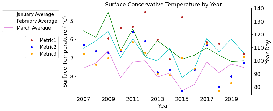
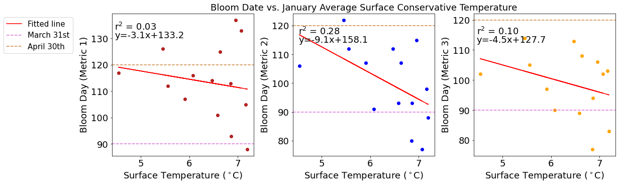
Monthly average surface temperature (January-March)
[13]:
fig,ax=plt.subplots(1,1,figsize=(12,5),constrained_layout=True)
p1=ax.plot(years,tempjan, '-',color='green',label='January Average')
p2=ax.plot(years,tempfeb, '-',color='c',label='February Average')
p3=ax.plot(years,tempmar, '-',color='orchid',label='March Average')
ax.set_ylabel('Surface Temperature ($^\circ$C)')
ax.set_xlabel('Year')
ax.set_title('Surface Conservative Temperature by Year')
ax.set_xticks([2007,2009,2011,2013,2015,2017,2019])
ax.legend(handles=[p1[0],p2[0],p3[0]],bbox_to_anchor=(-0.43, 1.0), loc='upper left')
ax.invert_yaxis()
ax1=ax.twinx()
p4=ax1.plot(years,yearday1, 'o',color='firebrick',label='Metric1')
p5=ax1.plot(years,yearday2, 'o',color='b',label='Metric2')
p6=ax1.plot(years,yearday3, 'o',color='orange',label='Metric3')
ax1.set_ylabel('Year Day')
ax1.legend(handles=[p4[0],p5[0],p6[0]],bbox_to_anchor=(-0.3, 0.7), loc='upper left')
# JAN
fig2,ax2=plt.subplots(1,3,figsize=(17,5),constrained_layout=True)
ax2[0].plot(tempjan,yearday1,'o',color='firebrick')
ax2[0].set_xlabel('Surface Temperature ($^\circ$C)')
ax2[0].set_ylabel('Bloom Day (Metric 1)')
y,r2,m,b=bloomdrivers.reg_r2(tempjan,yearday1)
ax2[0].plot(tempjan, y, 'r', label='Fitted line')
ax2[0].text(0.02, 0.9, '$\mathregular{r^2}$ = %.2f'%r2, transform=ax.transAxes)
ax2[0].text(0.02,0.83,f'y={round(m,1)}x+{round(b,1)}',horizontalalignment='left',verticalalignment='bottom',transform=ax.transAxes)
ax2[1].plot(tempjan,yearday2,'o',color='b')
ax2[1].set_xlabel('Surface Temperature ($^\circ$C)')
ax2[1].set_ylabel('Bloom Day (Metric 2)')
y,r2,m,b=bloomdrivers.reg_r2(tempjan,yearday2)
ax2[1].plot(tempjan, y, 'r', label='Fitted line')
ax2[1].text(0.65, 0.87, '$\mathregular{r^2}$ = %.2f'%r2, transform=ax.transAxes)
ax2[1].text(0.65,0.8,f'y={round(m,1)}x+{round(b,1)}',horizontalalignment='left',verticalalignment='bottom',transform=ax.transAxes)
ax2[2].plot(tempjan,yearday3,'o',color='orange')
ax2[2].set_xlabel('Surface Temperature ($^\circ$C)')
ax2[2].set_ylabel('Bloom Day (Metric 3)')
y,r2,m,b=bloomdrivers.reg_r2(tempjan,yearday3)
ax2[2].plot(tempjan, y, 'r', label='Fitted line')
ax2[2].text(1.26, 0.87, '$\mathregular{r^2}$ = %.2f'%r2, transform=ax.transAxes)
ax2[2].text(1.26,0.8,f'y={round(m,1)}x+{round(b,1)}',horizontalalignment='left',verticalalignment='bottom',transform=ax.transAxes)
ax2[1].set_title('Bloom Date vs. January Average Surface Conservative Temperature')
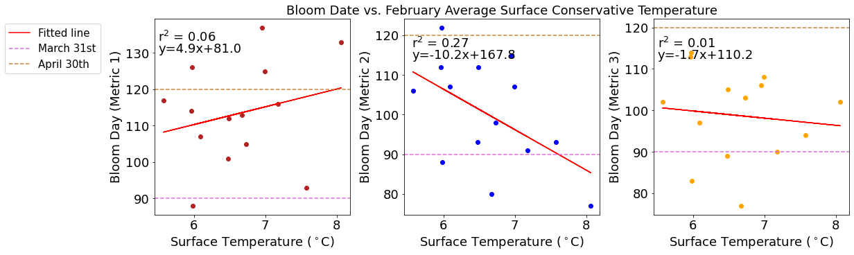
# FEB
fig3,ax3=plt.subplots(1,3,figsize=(17,5),constrained_layout=True)
ax3[0].plot(tempfeb,yearday1,'o',color='firebrick')
ax3[0].set_xlabel('Surface Temperature ($^\circ$C)')
ax3[0].set_ylabel('Bloom Day (Metric 1)')
y,r2,m,b=bloomdrivers.reg_r2(tempfeb,yearday1)
ax3[0].plot(tempfeb, y, 'r', label='Fitted line')
ax3[0].text(0.02, 0.9, '$\mathregular{r^2}$ = %.2f'%r2, transform=ax.transAxes)
ax3[0].text(0.02,0.83,f'y={round(m,1)}x+{round(b,1)}',horizontalalignment='left',verticalalignment='bottom',transform=ax.transAxes)
ax3[1].plot(tempfeb,yearday2,'o',color='b')
ax3[1].set_xlabel('Surface Temperature ($^\circ$C)')
ax3[1].set_ylabel('Bloom Day (Metric 2)')
y,r2,m,b=bloomdrivers.reg_r2(tempfeb,yearday2)
ax3[1].plot(tempfeb, y, 'r', label='Fitted line')
ax3[1].text(0.65, 0.87, '$\mathregular{r^2}$ = %.2f'%r2, transform=ax.transAxes)
ax3[1].text(0.65,0.8,f'y={round(m,1)}x+{round(b,1)}',horizontalalignment='left',verticalalignment='bottom',transform=ax.transAxes)
ax3[2].plot(tempfeb,yearday3,'o',color='orange')
ax3[2].set_xlabel('Surface Temperature ($^\circ$C)')
ax3[2].set_ylabel('Bloom Day (Metric 3)')
y,r2,m,b=bloomdrivers.reg_r2(tempfeb,yearday3)
ax3[2].plot(tempfeb, y, 'r', label='Fitted line')
ax3[2].text(1.26, 0.87, '$\mathregular{r^2}$ = %.2f'%r2, transform=ax.transAxes)
ax3[2].text(1.26,0.8,f'y={round(m,1)}x+{round(b,1)}',horizontalalignment='left',verticalalignment='bottom',transform=ax.transAxes)
ax3[1].set_title('Bloom Date vs. February Average Surface Conservative Temperature')
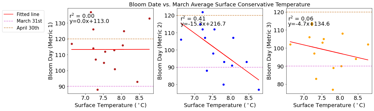
# MARCH
fig4,ax4=plt.subplots(1,3,figsize=(17,5),constrained_layout=True)
ax4[0].plot(tempmar,yearday1,'o',color='firebrick')
ax4[0].set_xlabel('Surface Temperature ($^\circ$C)')
ax4[0].set_ylabel('Bloom Day (Metric 1)')
y,r2,m,b=bloomdrivers.reg_r2(tempmar,yearday1)
ax4[0].plot(tempmar, y, 'r', label='Fitted line')
ax4[0].text(0.02, 0.9, '$\mathregular{r^2}$ = %.2f'%r2, transform=ax.transAxes)
ax4[0].text(0.02,0.83,f'y={round(m,1)}x+{round(b,1)}',horizontalalignment='left',verticalalignment='bottom',transform=ax.transAxes)
ax4[1].plot(tempmar,yearday2,'o',color='b')
ax4[1].set_xlabel('Surface Temperature ($^\circ$C)')
ax4[1].set_ylabel('Bloom Day (Metric 2)')
y,r2,m,b=bloomdrivers.reg_r2(tempmar,yearday2)
ax4[1].plot(tempmar, y, 'r', label='Fitted line')
ax4[1].text(0.65, 0.87, '$\mathregular{r^2}$ = %.2f'%r2, transform=ax.transAxes)
ax4[1].text(0.65,0.8,f'y={round(m,1)}x+{round(b,1)}',horizontalalignment='left',verticalalignment='bottom',transform=ax.transAxes)
ax4[2].plot(tempmar,yearday3,'o',color='orange')
ax4[2].set_xlabel('Surface Temperature ($^\circ$C)')
ax4[2].set_ylabel('Bloom Day (Metric 3)')
ax4[1].set_title('Bloom Date vs. March Average Surface Conservative Temperature')
y,r2,m,b=bloomdrivers.reg_r2(tempmar,yearday3)
ax4[2].plot(tempmar, y, 'r', label='Fitted line')
ax4[2].text(1.26, 0.87, '$\mathregular{r^2}$ = %.2f'%r2, transform=ax.transAxes)
ax4[2].text(1.26,0.8,f'y={round(m,1)}x+{round(b,1)}',horizontalalignment='left',verticalalignment='bottom',transform=ax.transAxes)
# Jan month lines
ax2[0].axhline(y=90, color='orchid', linestyle='--',label='March 31st')
ax2[0].axhline(y=120, color='peru', linestyle='--',label='April 30th')
#ax2[0].axhline(y=151, color='lime', linestyle='--',label='May 31st')
ax2[0].legend(bbox_to_anchor=(-0.25, 1.0))
ax2[1].axhline(y=90, color='orchid', linestyle='--')
ax2[2].axhline(y=90, color='orchid', linestyle='--',label='March 31st')
ax2[1].axhline(y=120, color='peru', linestyle='--')
ax2[2].axhline(y=120, color='peru', linestyle='--',label='April 30th')
# Feb month lines
ax3[0].axhline(y=90, color='orchid', linestyle='--',label='March 31st')
ax3[0].axhline(y=120, color='peru', linestyle='--',label='April 30th')
#ax3[0].axhline(y=151, color='lime', linestyle='--',label='May 31st')
ax3[0].legend(bbox_to_anchor=(-0.25, 1.0))
ax3[1].axhline(y=90, color='orchid', linestyle='--')
ax3[2].axhline(y=90, color='orchid', linestyle='--',label='March 31st')
ax3[1].axhline(y=120, color='peru', linestyle='--')
ax3[2].axhline(y=120, color='peru', linestyle='--',label='April 30th')
# March month lines
ax4[0].axhline(y=90, color='orchid', linestyle='--',label='March 31st')
ax4[0].axhline(y=120, color='peru', linestyle='--',label='April 30th')
#ax4[0].axhline(y=151, color='lime', linestyle='--',label='May 31st')
ax4[0].legend(bbox_to_anchor=(-0.25, 1.0))
ax4[1].axhline(y=90, color='orchid', linestyle='--')
ax4[2].axhline(y=90, color='orchid', linestyle='--',label='March 31st')
ax4[1].axhline(y=120, color='peru', linestyle='--')
ax4[2].axhline(y=120, color='peru', linestyle='--',label='April 30th')
#ax4[1].legend(handles=[p4[0],p5[0],p6[0]],bbox_to_anchor=(-1.7, 0.8), loc='upper left')
[13]:
<matplotlib.lines.Line2D at 0x7f70f9605760>
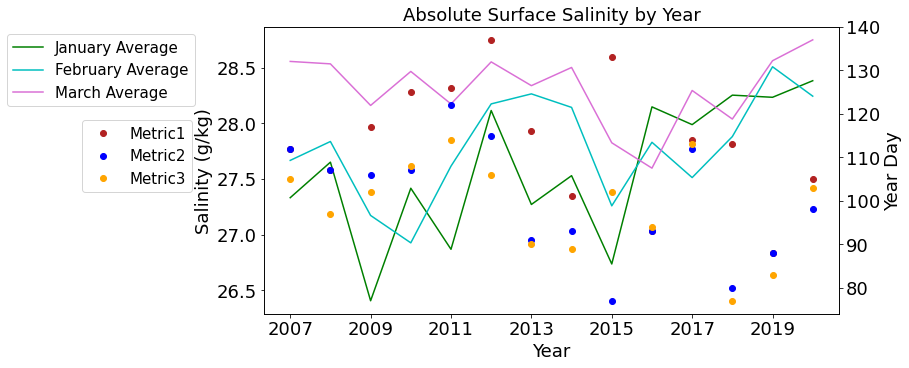
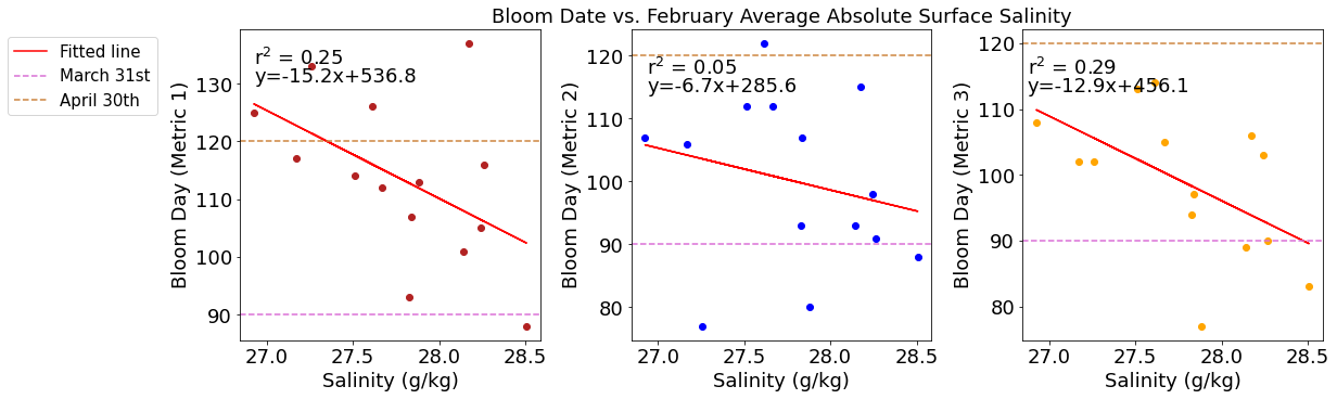
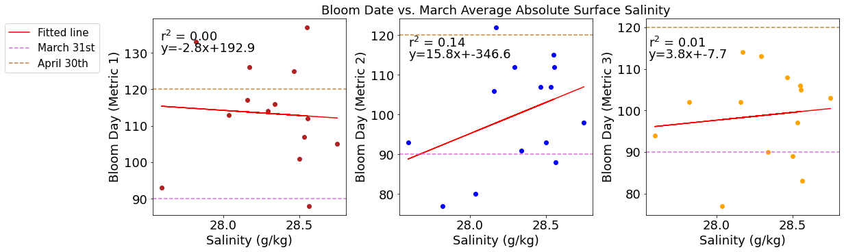
Monthly average surface salinity (January-March)
[29]:
fig,ax=plt.subplots(1,1,figsize=(12,5),constrained_layout=True)
p1=ax.plot(years,saljan, '-',color='green',label='January Average')
p2=ax.plot(years,salfeb, '-',color='c',label='February Average')
p3=ax.plot(years,salmar, '-',color='orchid',label='March Average')
ax.set_ylabel('Salinity (g/kg)')
ax.set_xlabel('Year')
ax.set_title('Absolute Surface Salinity by Year')
ax.set_xticks([2007,2009,2011,2013,2015,2017,2019])
ax.legend(handles=[p1[0],p2[0],p3[0]],bbox_to_anchor=(-0.46, 1.0), loc='upper left')
ax1=ax.twinx()
p4=ax1.plot(years,yearday1, 'o',color='firebrick',label='Metric1')
p5=ax1.plot(years,yearday2, 'o',color='b',label='Metric2')
p6=ax1.plot(years,yearday3, 'o',color='orange',label='Metric3')
ax1.set_ylabel('Year Day')
ax1.legend(handles=[p4[0],p5[0],p6[0]],bbox_to_anchor=(-0.33, 0.7), loc='upper left')
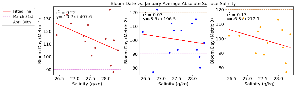
# JAN
fig2,ax2=plt.subplots(1,3,figsize=(17,5),constrained_layout=True)
ax2[0].plot(saljan,yearday1,'o',color='firebrick')
ax2[0].set_xlabel('Salinity (g/kg)')
ax2[0].set_ylabel('Bloom Day (Metric 1)')
y,r2,m,b=bloomdrivers.reg_r2(saljan,yearday1)
ax2[0].plot(saljan, y, 'r', label='Fitted line')
ax2[0].text(0.02, 0.9, '$\mathregular{r^2}$ = %.2f'%r2, transform=ax.transAxes)
ax2[0].text(0.02,0.83,f'y={round(m,1)}x+{round(b,1)}',horizontalalignment='left',verticalalignment='bottom',transform=ax.transAxes)
ax2[1].plot(saljan,yearday2,'o',color='b')
ax2[1].set_xlabel('Salinity (g/kg)')
ax2[1].set_ylabel('Bloom Day (Metric 2)')
y,r2,m,b=bloomdrivers.reg_r2(saljan,yearday2)
ax2[1].plot(saljan, y, 'r', label='Fitted line')
ax2[1].text(0.65, 0.87, '$\mathregular{r^2}$ = %.2f'%r2, transform=ax.transAxes)
ax2[1].text(0.65,0.8,f'y={round(m,1)}x+{round(b,1)}',horizontalalignment='left',verticalalignment='bottom',transform=ax.transAxes)
ax2[2].plot(saljan,yearday3,'o',color='orange')
ax2[2].set_xlabel('Salinity (g/kg)')
ax2[2].set_ylabel('Bloom Day (Metric 3)')
ax2[1].set_title('Bloom Date vs. January Average Absolute Surface Salinity')
y,r2,m,b=bloomdrivers.reg_r2(saljan,yearday3)
ax2[2].plot(saljan, y, 'r', label='Fitted line')
ax2[2].text(1.26, 0.87, '$\mathregular{r^2}$ = %.2f'%r2, transform=ax.transAxes)
ax2[2].text(1.26,0.8,f'y={round(m,1)}x+{round(b,1)}',horizontalalignment='left',verticalalignment='bottom',transform=ax.transAxes)
# FEB
fig3,ax3=plt.subplots(1,3,figsize=(17,5),constrained_layout=True)
ax3[0].plot(salfeb,yearday1,'o',color='firebrick')
ax3[0].set_xlabel('Salinity (g/kg)')
ax3[0].set_ylabel('Bloom Day (Metric 1)')
y,r2,m,b=bloomdrivers.reg_r2(salfeb,yearday1)
ax3[0].plot(salfeb, y, 'r', label='Fitted line')
ax3[0].text(0.02, 0.9, '$\mathregular{r^2}$ = %.2f'%r2, transform=ax.transAxes)
ax3[0].text(0.02,0.83,f'y={round(m,1)}x+{round(b,1)}',horizontalalignment='left',verticalalignment='bottom',transform=ax.transAxes)
ax3[1].plot(salfeb,yearday2,'o',color='b')
ax3[1].set_xlabel('Salinity (g/kg)')
ax3[1].set_ylabel('Bloom Day (Metric 2)')
y,r2,m,b=bloomdrivers.reg_r2(salfeb,yearday2)
ax3[1].plot(salfeb, y, 'r', label='Fitted line')
ax3[1].text(0.65, 0.87, '$\mathregular{r^2}$ = %.2f'%r2, transform=ax.transAxes)
ax3[1].text(0.65,0.8,f'y={round(m,1)}x+{round(b,1)}',horizontalalignment='left',verticalalignment='bottom',transform=ax.transAxes)
ax3[2].plot(salfeb,yearday3,'o',color='orange')
ax3[2].set_xlabel('Salinity (g/kg)')
ax3[2].set_ylabel('Bloom Day (Metric 3)')
ax3[1].set_title('Bloom Date vs. February Average Absolute Surface Salinity')
y,r2,m,b=bloomdrivers.reg_r2(salfeb,yearday3)
ax3[2].plot(salfeb, y, 'r', label='Fitted line')
ax3[2].text(1.26, 0.87, '$\mathregular{r^2}$ = %.2f'%r2, transform=ax.transAxes)
ax3[2].text(1.26,0.8,f'y={round(m,1)}x+{round(b,1)}',horizontalalignment='left',verticalalignment='bottom',transform=ax.transAxes)
# MAR
fig4,ax4=plt.subplots(1,3,figsize=(17,5),constrained_layout=True)
ax4[0].plot(salmar,yearday1,'o',color='firebrick')
ax4[0].set_xlabel('Salinity (g/kg)')
ax4[0].set_ylabel('Bloom Day (Metric 1)')
y,r2,m,b=bloomdrivers.reg_r2(salmar,yearday1)
ax4[0].plot(salmar, y, 'r', label='Fitted line')
ax4[0].text(0.02, 0.9, '$\mathregular{r^2}$ = %.2f'%r2, transform=ax.transAxes)
ax4[0].text(0.02,0.83,f'y={round(m,1)}x+{round(b,1)}',horizontalalignment='left',verticalalignment='bottom',transform=ax.transAxes)
ax4[1].plot(salmar,yearday2,'o',color='b')
ax4[1].set_xlabel('Salinity (g/kg)')
ax4[1].set_ylabel('Bloom Day (Metric 2)')
y,r2,m,b=bloomdrivers.reg_r2(salmar,yearday2)
ax4[1].plot(salmar, y, 'r', label='Fitted line')
ax4[1].text(0.65, 0.87, '$\mathregular{r^2}$ = %.2f'%r2, transform=ax.transAxes)
ax4[1].text(0.65,0.8,f'y={round(m,1)}x+{round(b,1)}',horizontalalignment='left',verticalalignment='bottom',transform=ax.transAxes)
ax4[2].plot(salmar,yearday3,'o',color='orange')
ax4[2].set_xlabel('Salinity (g/kg)')
ax4[2].set_ylabel('Bloom Day (Metric 3)')
ax4[1].set_title('Bloom Date vs. March Average Absolute Surface Salinity')
y,r2,m,b=bloomdrivers.reg_r2(salmar,yearday3)
ax4[2].plot(salmar, y, 'r', label='Fitted line')
ax4[2].text(1.26, 0.87, '$\mathregular{r^2}$ = %.2f'%r2, transform=ax.transAxes)
ax4[2].text(1.26,0.8,f'y={round(m,1)}x+{round(b,1)}',horizontalalignment='left',verticalalignment='bottom',transform=ax.transAxes)
# Jan month lines
ax2[0].axhline(y=90, color='orchid', linestyle='--',label='March 31st')
ax2[0].axhline(y=120, color='peru', linestyle='--',label='April 30th')
#ax2[0].axhline(y=151, color='lime', linestyle='--',label='May 31st')
ax2[0].legend(bbox_to_anchor=(-0.25, 1.0))
ax2[1].axhline(y=90, color='orchid', linestyle='--')
ax2[2].axhline(y=90, color='orchid', linestyle='--',label='March 31st')
ax2[1].axhline(y=120, color='peru', linestyle='--')
ax2[2].axhline(y=120, color='peru', linestyle='--',label='April 30th')
# Feb month lines
ax3[0].axhline(y=90, color='orchid', linestyle='--',label='March 31st')
ax3[0].axhline(y=120, color='peru', linestyle='--',label='April 30th')
#ax3[0].axhline(y=151, color='lime', linestyle='--',label='May 31st')
ax3[0].legend(bbox_to_anchor=(-0.25, 1.0))
ax3[1].axhline(y=90, color='orchid', linestyle='--')
ax3[2].axhline(y=90, color='orchid', linestyle='--',label='March 31st')
ax3[1].axhline(y=120, color='peru', linestyle='--')
ax3[2].axhline(y=120, color='peru', linestyle='--',label='April 30th')
# March month lines
ax4[0].axhline(y=90, color='orchid', linestyle='--',label='March 31st')
ax4[0].axhline(y=120, color='peru', linestyle='--',label='April 30th')
#ax4[0].axhline(y=151, color='lime', linestyle='--',label='May 31st')
ax4[0].legend(bbox_to_anchor=(-0.25, 1.0))
ax4[1].axhline(y=90, color='orchid', linestyle='--')
ax4[2].axhline(y=90, color='orchid', linestyle='--',label='March 31st')
ax4[1].axhline(y=120, color='peru', linestyle='--')
ax4[2].axhline(y=120, color='peru', linestyle='--',label='April 30th')
[29]:
<matplotlib.lines.Line2D at 0x7f70f89f7fd0>
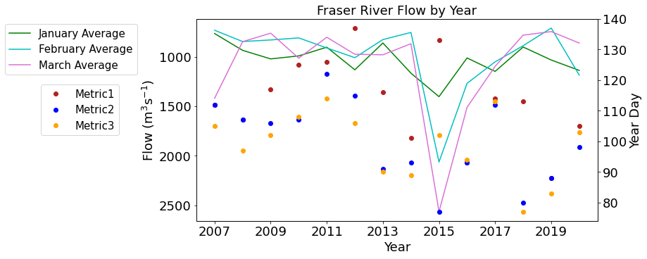
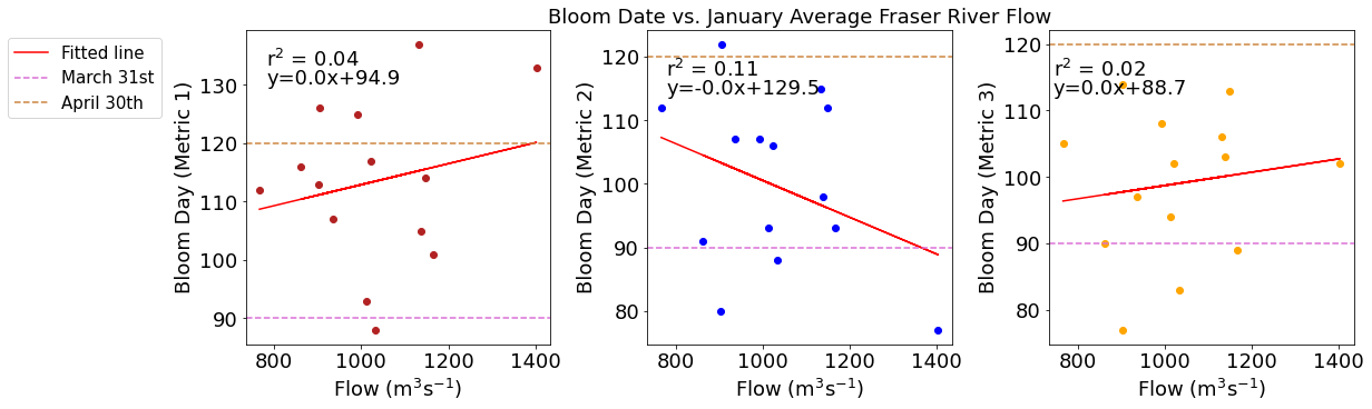
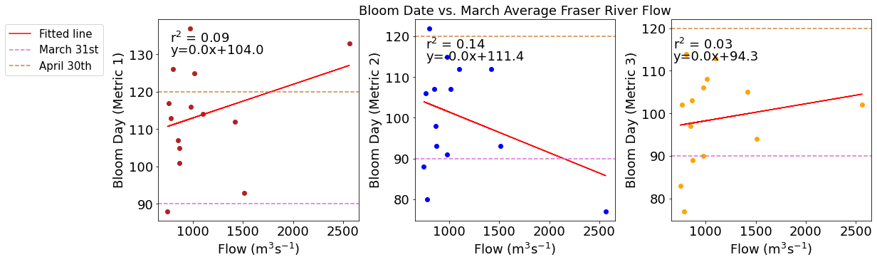
Monthly average Fraser river flow (January-March)
[15]:
fraseryears=years[:-1]
fig,ax=plt.subplots(1,1,figsize=(12,5),constrained_layout=True)
p1=ax.plot(years,fraserjan, '-',color='green',label='January Average')
p2=ax.plot(years,fraserfeb, '-',color='c',label='February Average')
p3=ax.plot(years,frasermar, '-',color='orchid',label='March Average')
ax.set_ylabel('Flow (m$^3$s$^{-1}$)')
ax.set_xlabel('Year')
ax.set_title('Fraser River Flow by Year')
ax.set_xticks([2007,2009,2011,2013,2015,2017,2019])
ax.legend(handles=[p1[0],p2[0],p3[0]],bbox_to_anchor=(-0.49, 1.0), loc='upper left')
ax.invert_yaxis()

ax1=ax.twinx()
p4=ax1.plot(years,yearday1, 'o',color='firebrick',label='Metric1')
p5=ax1.plot(years,yearday2, 'o',color='b',label='Metric2')
p6=ax1.plot(years,yearday3, 'o',color='orange',label='Metric3')
ax1.set_ylabel('Year Day')
ax1.legend(handles=[p4[0],p5[0],p6[0]],bbox_to_anchor=(-0.4, 0.7), loc='upper left')

# JAN
fig2,ax2=plt.subplots(1,3,figsize=(17,5),constrained_layout=True)
ax2[0].plot(fraserjan,yearday1,'o',color='firebrick')
ax2[0].set_xlabel('Flow (m$^3$s$^{-1}$)')
ax2[0].set_ylabel('Bloom Day (Metric 1)')
y,r2,m,b=bloomdrivers.reg_r2(fraserjan,yearday1)
ax2[0].plot(fraserjan, y, 'r', label='Fitted line')
ax2[0].text(0.02, 0.9, '$\mathregular{r^2}$ = %.2f'%r2, transform=ax.transAxes)
ax2[0].text(0.02,0.83,f'y={round(m,1)}x+{round(b,1)}',horizontalalignment='left',verticalalignment='bottom',transform=ax.transAxes)

ax2[1].plot(fraserjan,yearday2,'o',color='b')
ax2[1].set_xlabel('Flow (m$^3$s$^{-1}$)')
ax2[1].set_ylabel('Bloom Day (Metric 2)')
y,r2,m,b=bloomdrivers.reg_r2(fraserjan,yearday2)
ax2[1].plot(fraserjan, y, 'r', label='Fitted line')
ax2[1].text(0.65, 0.87, '$\mathregular{r^2}$ = %.2f'%r2, transform=ax.transAxes)
ax2[1].text(0.65,0.8,f'y={round(m,1)}x+{round(b,1)}',horizontalalignment='left',verticalalignment='bottom',transform=ax.transAxes)

ax2[2].plot(fraserjan,yearday3,'o',color='orange')
ax2[2].set_xlabel('Flow (m$^3$s$^{-1}$)')
ax2[2].set_ylabel('Bloom Day (Metric 3)')
ax2[1].set_title('Bloom Date vs. January Average Fraser River Flow')
y,r2,m,b=bloomdrivers.reg_r2(fraserjan,yearday3)
ax2[2].plot(fraserjan, y, 'r', label='Fitted line')
ax2[2].text(1.26, 0.87, '$\mathregular{r^2}$ = %.2f'%r2, transform=ax.transAxes)
ax2[2].text(1.26,0.8,f'y={round(m,1)}x+{round(b,1)}',horizontalalignment='left',verticalalignment='bottom',transform=ax.transAxes)

# FEB
fig3,ax3=plt.subplots(1,3,figsize=(17,5),constrained_layout=True)
ax3[0].plot(fraserfeb,yearday1,'o',color='firebrick')
ax3[0].set_xlabel('Flow (m$^3$s$^{-1}$)')
ax3[0].set_ylabel('Bloom Day (Metric 1)')
y,r2,m,b=bloomdrivers.reg_r2(fraserfeb,yearday1)
ax3[0].plot(fraserfeb, y, 'r', label='Fitted line')
ax3[0].text(0.02, 0.9, '$\mathregular{r^2}$ = %.2f'%r2, transform=ax.transAxes)
ax3[0].text(0.02,0.83,f'y={round(m,1)}x+{round(b,1)}',horizontalalignment='left',verticalalignment='bottom',transform=ax.transAxes)


ax3[1].plot(fraserfeb,yearday2,'o',color='b')
ax3[1].set_xlabel('Flow (m$^3$s$^{-1}$)')
ax3[1].set_ylabel('Bloom Day (Metric 2)')
y,r2,m,b=bloomdrivers.reg_r2(fraserfeb,yearday2)
ax3[1].plot(fraserfeb, y, 'r', label='Fitted line')
ax3[1].text(0.65, 0.87, '$\mathregular{r^2}$ = %.2f'%r2, transform=ax.transAxes)
ax3[1].text(0.65,0.8,f'y={round(m,1)}x+{round(b,1)}',horizontalalignment='left',verticalalignment='bottom',transform=ax.transAxes)

ax3[2].plot(fraserfeb,yearday3,'o',color='orange')
ax3[2].set_xlabel('Flow (m$^3$s$^{-1}$)')
ax3[2].set_ylabel('Bloom Day (Metric 3)')
ax3[1].set_title('Bloom Date vs. February Average Fraser River Flow')
y,r2,m,b=bloomdrivers.reg_r2(fraserfeb,yearday3)
ax3[2].plot(fraserfeb, y, 'r', label='Fitted line')
ax3[2].text(1.26, 0.87, '$\mathregular{r^2}$ = %.2f'%r2, transform=ax.transAxes)
ax3[2].text(1.26,0.8,f'y={round(m,1)}x+{round(b,1)}',horizontalalignment='left',verticalalignment='bottom',transform=ax.transAxes)

# MAR
fig4,ax4=plt.subplots(1,3,figsize=(17,5),constrained_layout=True)
ax4[0].plot(frasermar,yearday1,'o',color='firebrick')
ax4[0].set_xlabel('Flow (m$^3$s$^{-1}$)')
ax4[0].set_ylabel('Bloom Day (Metric 1)')
y,r2,m,b=bloomdrivers.reg_r2(frasermar,yearday1)
ax4[0].plot(frasermar, y, 'r', label='Fitted line')
ax4[0].text(0.02, 0.9, '$\mathregular{r^2}$ = %.2f'%r2, transform=ax.transAxes)
ax4[0].text(0.02,0.83,f'y={round(m,1)}x+{round(b,1)}',horizontalalignment='left',verticalalignment='bottom',transform=ax.transAxes)

ax4[1].plot(frasermar,yearday2,'o',color='b')
ax4[1].set_xlabel('Flow (m$^3$s$^{-1}$)')
ax4[1].set_ylabel('Bloom Day (Metric 2)')
y,r2,m,b=bloomdrivers.reg_r2(frasermar,yearday2)
ax4[1].plot(frasermar, y, 'r', label='Fitted line')
ax4[1].text(0.65, 0.87, '$\mathregular{r^2}$ = %.2f'%r2, transform=ax.transAxes)
ax4[1].text(0.65,0.8,f'y={round(m,1)}x+{round(b,1)}',horizontalalignment='left',verticalalignment='bottom',transform=ax.transAxes)

ax4[2].plot(frasermar,yearday3,'o',color='orange')
ax4[2].set_xlabel('Flow (m$^3$s$^{-1}$)')
ax4[2].set_ylabel('Bloom Day (Metric 3)')
ax4[1].set_title('Bloom Date vs. March Average Fraser River Flow')
y,r2,m,b=bloomdrivers.reg_r2(frasermar,yearday3)
ax4[2].plot(frasermar, y, 'r', label='Fitted line')
ax4[2].text(1.26, 0.87, '$\mathregular{r^2}$ = %.2f'%r2, transform=ax.transAxes)
ax4[2].text(1.26,0.8,f'y={round(m,1)}x+{round(b,1)}',horizontalalignment='left',verticalalignment='bottom',transform=ax.transAxes)

# Jan month lines
ax2[0].axhline(y=90, color='orchid', linestyle='--',label='March 31st')
ax2[0].axhline(y=120, color='peru', linestyle='--',label='April 30th')
ax2[0].legend(bbox_to_anchor=(-0.25, 1.0))
ax2[1].axhline(y=90, color='orchid', linestyle='--')
ax2[2].axhline(y=90, color='orchid', linestyle='--',label='March 31st')
ax2[1].axhline(y=120, color='peru', linestyle='--')
ax2[2].axhline(y=120, color='peru', linestyle='--',label='April 30th')
# Feb month lines
ax3[0].axhline(y=90, color='orchid', linestyle='--',label='March 31st')
ax3[0].axhline(y=120, color='peru', linestyle='--',label='April 30th')
ax3[0].legend(bbox_to_anchor=(-0.25, 1.0))
ax3[1].axhline(y=90, color='orchid', linestyle='--')
ax3[2].axhline(y=90, color='orchid', linestyle='--',label='March 31st')
ax3[1].axhline(y=120, color='peru', linestyle='--')
ax3[2].axhline(y=120, color='peru', linestyle='--',label='April 30th')
# March month lines
ax4[0].axhline(y=90, color='orchid', linestyle='--',label='March 31st')
ax4[0].axhline(y=120, color='peru', linestyle='--',label='April 30th')
ax4[0].legend(bbox_to_anchor=(-0.25, 1.0))
ax4[1].axhline(y=90, color='orchid', linestyle='--')
ax4[2].axhline(y=90, color='orchid', linestyle='--',label='March 31st')
ax4[1].axhline(y=120, color='peru', linestyle='--')
ax4[2].axhline(y=120, color='peru', linestyle='--',label='April 30th')
#ax4[1].legend(handles=[p4[0],p5[0],p6[0]],bbox_to_anchor=(-1.7, 0.8), loc='upper left')
[15]:
<matplotlib.lines.Line2D at 0x7f70f974f970>

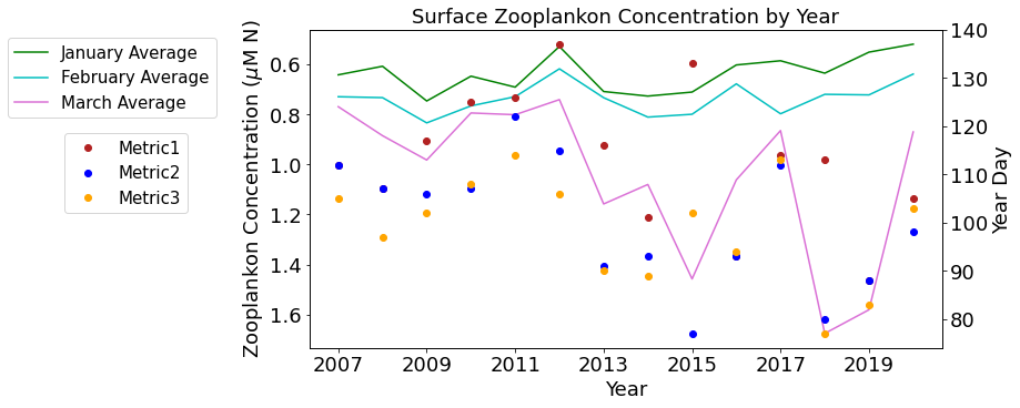
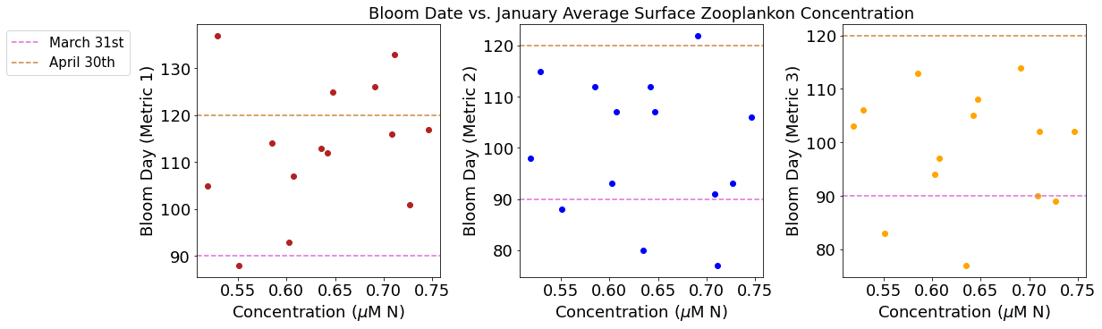
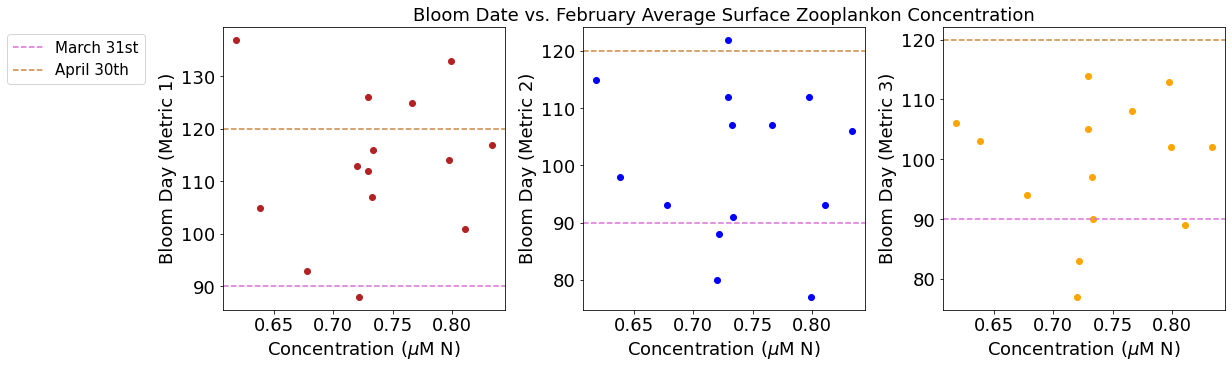
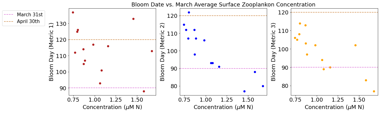
Monthly average surface zooplankton concentration (January-March)
[16]:
fig,ax=plt.subplots(1,1,figsize=(12,5),constrained_layout=True)
p1=ax.plot(years,zoojan, '-',color='green',label='January Average')
p2=ax.plot(years,zoofeb, '-',color='c',label='February Average')
p3=ax.plot(years,zoomar, '-',color='orchid',label='March Average')
ax.set_ylabel('Zooplankon Concentration ($\mu$M N)')
ax.set_xlabel('Year')
ax.set_title('Surface Zooplankon Concentration by Year')
ax.set_xticks([2007,2009,2011,2013,2015,2017,2019])
ax.legend(handles=[p1[0],p2[0],p3[0]],bbox_to_anchor=(-0.49, 1.0), loc='upper left')
ax.invert_yaxis()

ax1=ax.twinx()
p4=ax1.plot(years,yearday1, 'o',color='firebrick',label='Metric1')
p5=ax1.plot(years,yearday2, 'o',color='b',label='Metric2')
p6=ax1.plot(years,yearday3, 'o',color='orange',label='Metric3')
ax1.set_ylabel('Year Day')
ax1.legend(handles=[p4[0],p5[0],p6[0]],bbox_to_anchor=(-0.4, 0.7), loc='upper left')

fig2,ax2=plt.subplots(1,3,figsize=(17,5),constrained_layout=True)
ax2[0].plot(zoojan,yearday1,'o',color='firebrick')
ax2[0].set_xlabel('Concentration ($\mu$M N)')
ax2[0].set_ylabel('Bloom Day (Metric 1)')
ax2[1].plot(zoojan,yearday2,'o',color='b')
ax2[1].set_xlabel('Concentration ($\mu$M N)')
ax2[1].set_ylabel('Bloom Day (Metric 2)')
ax2[2].plot(zoojan,yearday3,'o',color='orange')
ax2[2].set_xlabel('Concentration ($\mu$M N)')
ax2[2].set_ylabel('Bloom Day (Metric 3)')
ax2[1].set_title('Bloom Date vs. January Average Surface Zooplankon Concentration')


fig3,ax3=plt.subplots(1,3,figsize=(17,5),constrained_layout=True)
ax3[0].plot(zoofeb,yearday1,'o',color='firebrick')
ax3[0].set_xlabel('Concentration ($\mu$M N)')
ax3[0].set_ylabel('Bloom Day (Metric 1)')
ax3[1].plot(zoofeb,yearday2,'o',color='b')
ax3[1].set_xlabel('Concentration ($\mu$M N)')
ax3[1].set_ylabel('Bloom Day (Metric 2)')
ax3[2].plot(zoofeb,yearday3,'o',color='orange')
ax3[2].set_xlabel('Concentration ($\mu$M N)')
ax3[2].set_ylabel('Bloom Day (Metric 3)')
ax3[1].set_title('Bloom Date vs. February Average Surface Zooplankon Concentration')


fig4,ax4=plt.subplots(1,3,figsize=(17,5),constrained_layout=True)
ax4[0].plot(zoomar,yearday1,'o',color='firebrick')
ax4[0].set_xlabel('Concentration ($\mu$M N)')
ax4[0].set_ylabel('Bloom Day (Metric 1)')
ax4[1].plot(zoomar,yearday2,'o',color='b')
ax4[1].set_xlabel('Concentration ($\mu$M N)')
ax4[1].set_ylabel('Bloom Day (Metric 2)')
ax4[2].plot(zoomar,yearday3,'o',color='orange')
ax4[2].set_xlabel('Concentration ($\mu$M N)')
ax4[2].set_ylabel('Bloom Day (Metric 3)')
ax4[1].set_title('Bloom Date vs. March Average Surface Zooplankon Concentration')


# Jan month lines
ax2[0].axhline(y=90, color='orchid', linestyle='--',label='March 31st')
ax2[0].axhline(y=120, color='peru', linestyle='--',label='April 30th')
#ax2[0].axhline(y=151, color='lime', linestyle='--',label='May 31st')
ax2[0].legend(bbox_to_anchor=(-0.25, 1.0))
ax2[1].axhline(y=90, color='orchid', linestyle='--')
ax2[2].axhline(y=90, color='orchid', linestyle='--',label='March 31st')
ax2[1].axhline(y=120, color='peru', linestyle='--')
ax2[2].axhline(y=120, color='peru', linestyle='--',label='April 30th')
# Feb month lines
ax3[0].axhline(y=90, color='orchid', linestyle='--',label='March 31st')
ax3[0].axhline(y=120, color='peru', linestyle='--',label='April 30th')
#ax3[0].axhline(y=151, color='lime', linestyle='--',label='May 31st')
ax3[0].legend(bbox_to_anchor=(-0.25, 1.0))
ax3[1].axhline(y=90, color='orchid', linestyle='--')
ax3[2].axhline(y=90, color='orchid', linestyle='--',label='March 31st')
ax3[1].axhline(y=120, color='peru', linestyle='--')
ax3[2].axhline(y=120, color='peru', linestyle='--',label='April 30th')
# March month lines
ax4[0].axhline(y=90, color='orchid', linestyle='--',label='March 31st')
ax4[0].axhline(y=120, color='peru', linestyle='--',label='April 30th')
#ax4[0].axhline(y=151, color='lime', linestyle='--',label='May 31st')
ax4[0].legend(bbox_to_anchor=(-0.25, 1.0))
ax4[1].axhline(y=90, color='orchid', linestyle='--')
ax4[2].axhline(y=90, color='orchid', linestyle='--',label='March 31st')
ax4[1].axhline(y=120, color='peru', linestyle='--')
ax4[2].axhline(y=120, color='peru', linestyle='--',label='April 30th')
[16]:
<matplotlib.lines.Line2D at 0x7f70f98a4c70>
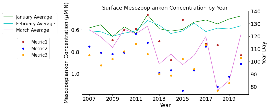
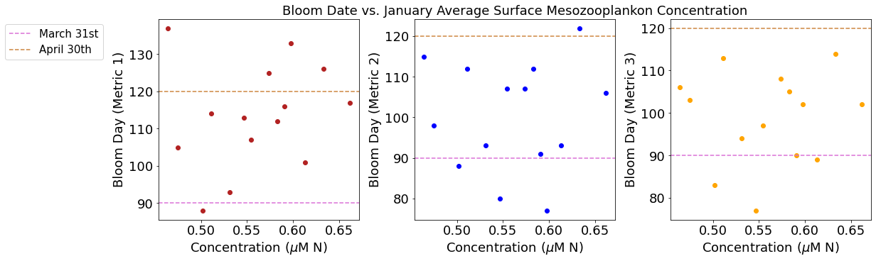
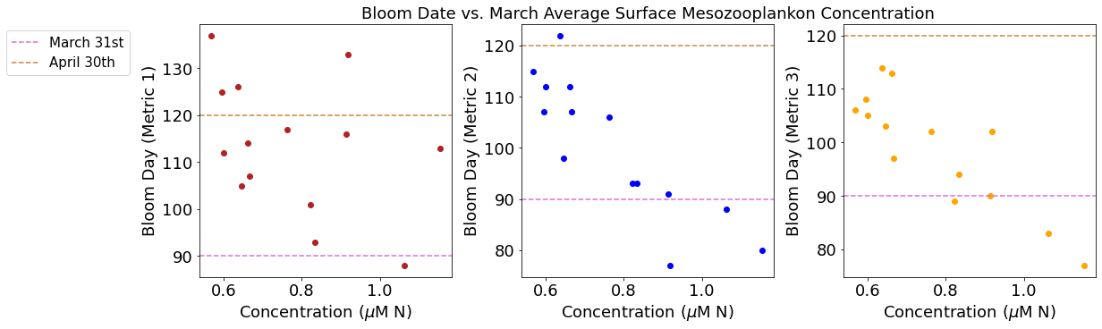
Monthly average surface mesozooplankton concentration (January-March)
[17]:
fig,ax=plt.subplots(1,1,figsize=(12,5),constrained_layout=True)
p1=ax.plot(years,mesozoojan, '-',color='green',label='January Average')
p2=ax.plot(years,mesozoofeb, '-',color='c',label='February Average')
p3=ax.plot(years,mesozoomar, '-',color='orchid',label='March Average')
ax.set_ylabel('Mesozooplankon Concentration ($\mu$M N)')
ax.set_xlabel('Year')
ax.set_title('Surface Mesozooplankon Concentration by Year')
ax.set_xticks([2007,2009,2011,2013,2015,2017,2019])
ax.legend(handles=[p1[0],p2[0],p3[0]],bbox_to_anchor=(-0.49, 1.0), loc='upper left')
ax.invert_yaxis()
ax1=ax.twinx()
p4=ax1.plot(years,yearday1, 'o',color='firebrick',label='Metric1')
p5=ax1.plot(years,yearday2, 'o',color='b',label='Metric2')
p6=ax1.plot(years,yearday3, 'o',color='orange',label='Metric3')
ax1.set_ylabel('Year Day')
ax1.legend(handles=[p4[0],p5[0],p6[0]],bbox_to_anchor=(-0.4, 0.7), loc='upper left')
fig2,ax2=plt.subplots(1,3,figsize=(17,5),constrained_layout=True)
ax2[0].plot(mesozoojan,yearday1,'o',color='firebrick')
ax2[0].set_xlabel('Concentration ($\mu$M N)')
ax2[0].set_ylabel('Bloom Day (Metric 1)')
ax2[1].plot(mesozoojan,yearday2,'o',color='b')
ax2[1].set_xlabel('Concentration ($\mu$M N)')
ax2[1].set_ylabel('Bloom Day (Metric 2)')
ax2[2].plot(mesozoojan,yearday3,'o',color='orange')
ax2[2].set_xlabel('Concentration ($\mu$M N)')
ax2[2].set_ylabel('Bloom Day (Metric 3)')
ax2[1].set_title('Bloom Date vs. January Average Surface Mesozooplankon Concentration')
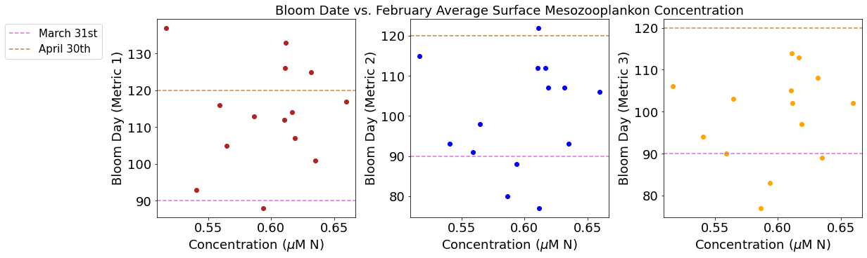
fig3,ax3=plt.subplots(1,3,figsize=(17,5),constrained_layout=True)
ax3[0].plot(mesozoofeb,yearday1,'o',color='firebrick')
ax3[0].set_xlabel('Concentration ($\mu$M N)')
ax3[0].set_ylabel('Bloom Day (Metric 1)')
ax3[1].plot(mesozoofeb,yearday2,'o',color='b')
ax3[1].set_xlabel('Concentration ($\mu$M N)')
ax3[1].set_ylabel('Bloom Day (Metric 2)')
ax3[2].plot(mesozoofeb,yearday3,'o',color='orange')
ax3[2].set_xlabel('Concentration ($\mu$M N)')
ax3[2].set_ylabel('Bloom Day (Metric 3)')
ax3[1].set_title('Bloom Date vs. February Average Surface Mesozooplankon Concentration')
fig4,ax4=plt.subplots(1,3,figsize=(17,5),constrained_layout=True)
ax4[0].plot(mesozoomar,yearday1,'o',color='firebrick')
ax4[0].set_xlabel('Concentration ($\mu$M N)')
ax4[0].set_ylabel('Bloom Day (Metric 1)')
ax4[1].plot(mesozoomar,yearday2,'o',color='b')
ax4[1].set_xlabel('Concentration ($\mu$M N)')
ax4[1].set_ylabel('Bloom Day (Metric 2)')
ax4[2].plot(mesozoomar,yearday3,'o',color='orange')
ax4[2].set_xlabel('Concentration ($\mu$M N)')
ax4[2].set_ylabel('Bloom Day (Metric 3)')
ax4[1].set_title('Bloom Date vs. March Average Surface Mesozooplankon Concentration')
# Jan month lines
ax2[0].axhline(y=90, color='orchid', linestyle='--',label='March 31st')
ax2[0].axhline(y=120, color='peru', linestyle='--',label='April 30th')
#ax2[0].axhline(y=151, color='lime', linestyle='--',label='May 31st')
ax2[0].legend(bbox_to_anchor=(-0.25, 1.0))
ax2[1].axhline(y=90, color='orchid', linestyle='--')
ax2[2].axhline(y=90, color='orchid', linestyle='--',label='March 31st')
ax2[1].axhline(y=120, color='peru', linestyle='--')
ax2[2].axhline(y=120, color='peru', linestyle='--',label='April 30th')
# Feb month lines
ax3[0].axhline(y=90, color='orchid', linestyle='--',label='March 31st')
ax3[0].axhline(y=120, color='peru', linestyle='--',label='April 30th')
#ax3[0].axhline(y=151, color='lime', linestyle='--',label='May 31st')
ax3[0].legend(bbox_to_anchor=(-0.25, 1.0))
ax3[1].axhline(y=90, color='orchid', linestyle='--')
ax3[2].axhline(y=90, color='orchid', linestyle='--',label='March 31st')
ax3[1].axhline(y=120, color='peru', linestyle='--')
ax3[2].axhline(y=120, color='peru', linestyle='--',label='April 30th')
# March month lines
ax4[0].axhline(y=90, color='orchid', linestyle='--',label='March 31st')
ax4[0].axhline(y=120, color='peru', linestyle='--',label='April 30th')
#ax4[0].axhline(y=151, color='lime', linestyle='--',label='May 31st')
ax4[0].legend(bbox_to_anchor=(-0.25, 1.0))
ax4[1].axhline(y=90, color='orchid', linestyle='--')
ax4[2].axhline(y=90, color='orchid', linestyle='--',label='March 31st')
ax4[1].axhline(y=120, color='peru', linestyle='--')
ax4[2].axhline(y=120, color='peru', linestyle='--',label='April 30th')
[17]:
<matplotlib.lines.Line2D at 0x7f70f9894fd0>
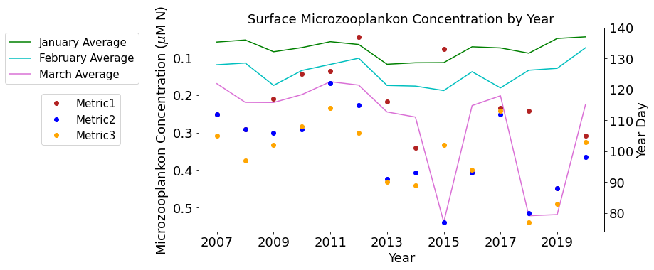
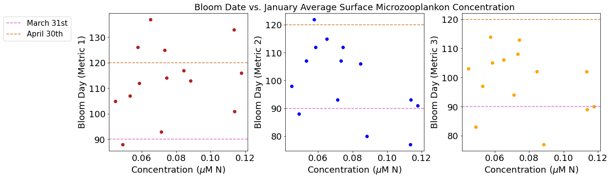
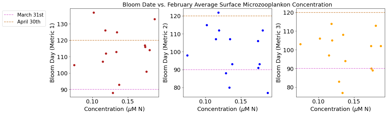
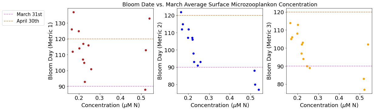
Monthly average surface microzooplankton concentration (January-March)
[18]:
fig,ax=plt.subplots(1,1,figsize=(12,5),constrained_layout=True)
p1=ax.plot(years,microzoojan, '-',color='green',label='January Average')
p2=ax.plot(years,microzoofeb, '-',color='c',label='February Average')
p3=ax.plot(years,microzoomar, '-',color='orchid',label='March Average')
ax.set_ylabel('Microzooplankon Concentration ($\mu$M N)')
ax.set_xlabel('Year')
ax.set_title('Surface Microzooplankon Concentration by Year')
ax.set_xticks([2007,2009,2011,2013,2015,2017,2019])
ax.legend(handles=[p1[0],p2[0],p3[0]],bbox_to_anchor=(-0.49, 1.0), loc='upper left')
ax.invert_yaxis()

ax1=ax.twinx()
p4=ax1.plot(years,yearday1, 'o',color='firebrick',label='Metric1')
p5=ax1.plot(years,yearday2, 'o',color='b',label='Metric2')
p6=ax1.plot(years,yearday3, 'o',color='orange',label='Metric3')
ax1.set_ylabel('Year Day')
ax1.legend(handles=[p4[0],p5[0],p6[0]],bbox_to_anchor=(-0.4, 0.7), loc='upper left')

fig2,ax2=plt.subplots(1,3,figsize=(17,5),constrained_layout=True)
ax2[0].plot(microzoojan,yearday1,'o',color='firebrick')
ax2[0].set_xlabel('Concentration ($\mu$M N)')
ax2[0].set_ylabel('Bloom Day (Metric 1)')
ax2[1].plot(microzoojan,yearday2,'o',color='b')
ax2[1].set_xlabel('Concentration ($\mu$M N)')
ax2[1].set_ylabel('Bloom Day (Metric 2)')
ax2[2].plot(microzoojan,yearday3,'o',color='orange')
ax2[2].set_xlabel('Concentration ($\mu$M N)')
ax2[2].set_ylabel('Bloom Day (Metric 3)')
ax2[1].set_title('Bloom Date vs. January Average Surface Microzooplankon Concentration')


fig3,ax3=plt.subplots(1,3,figsize=(17,5),constrained_layout=True)
ax3[0].plot(microzoofeb,yearday1,'o',color='firebrick')
ax3[0].set_xlabel('Concentration ($\mu$M N)')
ax3[0].set_ylabel('Bloom Day (Metric 1)')
ax3[1].plot(microzoofeb,yearday2,'o',color='b')
ax3[1].set_xlabel('Concentration ($\mu$M N)')
ax3[1].set_ylabel('Bloom Day (Metric 2)')
ax3[2].plot(microzoofeb,yearday3,'o',color='orange')
ax3[2].set_xlabel('Concentration ($\mu$M N)')
ax3[2].set_ylabel('Bloom Day (Metric 3)')
ax3[1].set_title('Bloom Date vs. February Average Surface Microzooplankon Concentration')

fig4,ax4=plt.subplots(1,3,figsize=(17,5),constrained_layout=True)
ax4[0].plot(microzoomar,yearday1,'o',color='firebrick')
ax4[0].set_xlabel('Concentration ($\mu$M N)')
ax4[0].set_ylabel('Bloom Day (Metric 1)')
ax4[1].plot(microzoomar,yearday2,'o',color='b')
ax4[1].set_xlabel('Concentration ($\mu$M N)')
ax4[1].set_ylabel('Bloom Day (Metric 2)')
ax4[2].plot(microzoomar,yearday3,'o',color='orange')
ax4[2].set_xlabel('Concentration ($\mu$M N)')
ax4[2].set_ylabel('Bloom Day (Metric 3)')
ax4[1].set_title('Bloom Date vs. March Average Surface Microzooplankon Concentration')


# Jan month lines
ax2[0].axhline(y=90, color='orchid', linestyle='--',label='March 31st')
ax2[0].axhline(y=120, color='peru', linestyle='--',label='April 30th')
#ax2[0].axhline(y=151, color='lime', linestyle='--',label='May 31st')
ax2[0].legend(bbox_to_anchor=(-0.25, 1.0))
ax2[1].axhline(y=90, color='orchid', linestyle='--')
ax2[2].axhline(y=90, color='orchid', linestyle='--',label='March 31st')
ax2[1].axhline(y=120, color='peru', linestyle='--')
ax2[2].axhline(y=120, color='peru', linestyle='--',label='April 30th')
# Feb month lines
ax3[0].axhline(y=90, color='orchid', linestyle='--',label='March 31st')
ax3[0].axhline(y=120, color='peru', linestyle='--',label='April 30th')
#ax3[0].axhline(y=151, color='lime', linestyle='--',label='May 31st')
ax3[0].legend(bbox_to_anchor=(-0.25, 1.0))
ax3[1].axhline(y=90, color='orchid', linestyle='--')
ax3[2].axhline(y=90, color='orchid', linestyle='--',label='March 31st')
ax3[1].axhline(y=120, color='peru', linestyle='--')
ax3[2].axhline(y=120, color='peru', linestyle='--',label='April 30th')
# March month lines
ax4[0].axhline(y=90, color='orchid', linestyle='--',label='March 31st')
ax4[0].axhline(y=120, color='peru', linestyle='--',label='April 30th')
#ax4[0].axhline(y=151, color='lime', linestyle='--',label='May 31st')
ax4[0].legend(bbox_to_anchor=(-0.25, 1.0))
ax4[1].axhline(y=90, color='orchid', linestyle='--')
ax4[2].axhline(y=90, color='orchid', linestyle='--',label='March 31st')
ax4[1].axhline(y=120, color='peru', linestyle='--')
ax4[2].axhline(y=120, color='peru', linestyle='--',label='April 30th')
[18]:
<matplotlib.lines.Line2D at 0x7f7109e86c10>
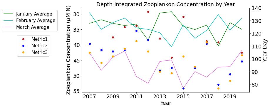
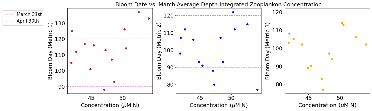
Monthly average depth-integrated zooplankton concentration (January-March)
[19]:
fig,ax=plt.subplots(1,1,figsize=(12,5),constrained_layout=True)
p1=ax.plot(years,intzoojan, '-',color='green',label='January Average')
p2=ax.plot(years,intzoofeb, '-',color='c',label='February Average')
p3=ax.plot(years,intzoomar, '-',color='orchid',label='March Average')
ax.set_ylabel('Zooplankon Concentration ($\mu$M N)')
ax.set_xlabel('Year')
ax.set_title('Depth-integrated Zooplankon Concentration by Year')
ax.set_xticks([2007,2009,2011,2013,2015,2017,2019])
ax.legend(handles=[p1[0],p2[0],p3[0]],bbox_to_anchor=(-0.49, 1.0), loc='upper left')
ax.invert_yaxis()
ax1=ax.twinx()
p4=ax1.plot(years,yearday1, 'o',color='firebrick',label='Metric1')
p5=ax1.plot(years,yearday2, 'o',color='b',label='Metric2')
p6=ax1.plot(years,yearday3, 'o',color='orange',label='Metric3')
ax1.set_ylabel('Year Day')
ax1.legend(handles=[p4[0],p5[0],p6[0]],bbox_to_anchor=(-0.4, 0.7), loc='upper left')
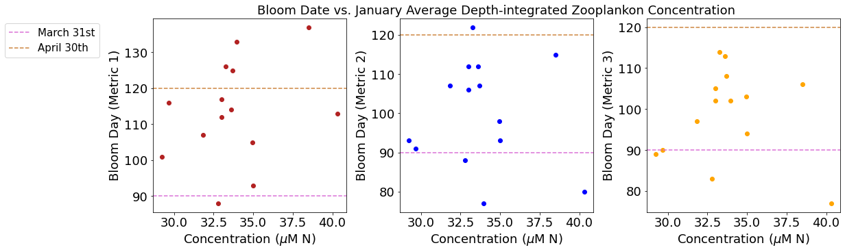
fig2,ax2=plt.subplots(1,3,figsize=(17,5),constrained_layout=True)
ax2[0].plot(intzoojan,yearday1,'o',color='firebrick')
ax2[0].set_xlabel('Concentration ($\mu$M N)')
ax2[0].set_ylabel('Bloom Day (Metric 1)')
ax2[1].plot(intzoojan,yearday2,'o',color='b')
ax2[1].set_xlabel('Concentration ($\mu$M N)')
ax2[1].set_ylabel('Bloom Day (Metric 2)')
ax2[2].plot(intzoojan,yearday3,'o',color='orange')
ax2[2].set_xlabel('Concentration ($\mu$M N)')
ax2[2].set_ylabel('Bloom Day (Metric 3)')
ax2[1].set_title('Bloom Date vs. January Average Depth-integrated Zooplankon Concentration')
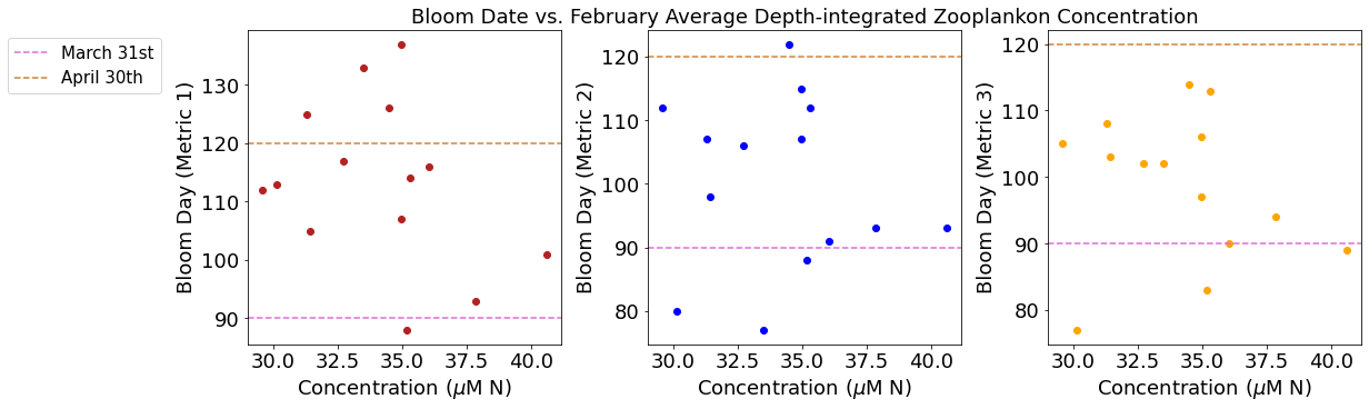
fig3,ax3=plt.subplots(1,3,figsize=(17,5),constrained_layout=True)
ax3[0].plot(intzoofeb,yearday1,'o',color='firebrick')
ax3[0].set_xlabel('Concentration ($\mu$M N)')
ax3[0].set_ylabel('Bloom Day (Metric 1)')
ax3[1].plot(intzoofeb,yearday2,'o',color='b')
ax3[1].set_xlabel('Concentration ($\mu$M N)')
ax3[1].set_ylabel('Bloom Day (Metric 2)')
ax3[2].plot(intzoofeb,yearday3,'o',color='orange')
ax3[2].set_xlabel('Concentration ($\mu$M N)')
ax3[2].set_ylabel('Bloom Day (Metric 3)')
ax3[1].set_title('Bloom Date vs. February Average Depth-integrated Zooplankon Concentration')
fig4,ax4=plt.subplots(1,3,figsize=(17,5),constrained_layout=True)
ax4[0].plot(intzoomar,yearday1,'o',color='firebrick')
ax4[0].set_xlabel('Concentration ($\mu$M N)')
ax4[0].set_ylabel('Bloom Day (Metric 1)')
ax4[1].plot(intzoomar,yearday2,'o',color='b')
ax4[1].set_xlabel('Concentration ($\mu$M N)')
ax4[1].set_ylabel('Bloom Day (Metric 2)')
ax4[2].plot(intzoomar,yearday3,'o',color='orange')
ax4[2].set_xlabel('Concentration ($\mu$M N)')
ax4[2].set_ylabel('Bloom Day (Metric 3)')
ax4[1].set_title('Bloom Date vs. March Average Depth-integrated Zooplankon Concentration')
# Jan month lines
ax2[0].axhline(y=90, color='orchid', linestyle='--',label='March 31st')
ax2[0].axhline(y=120, color='peru', linestyle='--',label='April 30th')
#ax2[0].axhline(y=151, color='lime', linestyle='--',label='May 31st')
ax2[0].legend(bbox_to_anchor=(-0.25, 1.0))
ax2[1].axhline(y=90, color='orchid', linestyle='--')
ax2[2].axhline(y=90, color='orchid', linestyle='--',label='March 31st')
ax2[1].axhline(y=120, color='peru', linestyle='--')
ax2[2].axhline(y=120, color='peru', linestyle='--',label='April 30th')
# Feb month lines
ax3[0].axhline(y=90, color='orchid', linestyle='--',label='March 31st')
ax3[0].axhline(y=120, color='peru', linestyle='--',label='April 30th')
#ax3[0].axhline(y=151, color='lime', linestyle='--',label='May 31st')
ax3[0].legend(bbox_to_anchor=(-0.25, 1.0))
ax3[1].axhline(y=90, color='orchid', linestyle='--')
ax3[2].axhline(y=90, color='orchid', linestyle='--',label='March 31st')
ax3[1].axhline(y=120, color='peru', linestyle='--')
ax3[2].axhline(y=120, color='peru', linestyle='--',label='April 30th')
# March month lines
ax4[0].axhline(y=90, color='orchid', linestyle='--',label='March 31st')
ax4[0].axhline(y=120, color='peru', linestyle='--',label='April 30th')
#ax4[0].axhline(y=151, color='lime', linestyle='--',label='May 31st')
ax4[0].legend(bbox_to_anchor=(-0.25, 1.0))
ax4[1].axhline(y=90, color='orchid', linestyle='--')
ax4[2].axhline(y=90, color='orchid', linestyle='--',label='March 31st')
ax4[1].axhline(y=120, color='peru', linestyle='--')
ax4[2].axhline(y=120, color='peru', linestyle='--',label='April 30th')
[19]:
<matplotlib.lines.Line2D at 0x7f70f8f2ffd0>
Monthly average depth-integrated mesozooplankton concentration (January-March)
[20]:
fig,ax=plt.subplots(1,1,figsize=(12,5),constrained_layout=True)
p1=ax.plot(years,intmesozoojan, '-',color='green',label='January Average')
p2=ax.plot(years,intmesozoofeb, '-',color='c',label='February Average')
p3=ax.plot(years,intmesozoomar, '-',color='orchid',label='March Average')
ax.set_ylabel('Mesozooplankon Concentration ($\mu$M N)')
ax.set_xlabel('Year')
ax.set_title('Depth-integrated Mesozooplankon Concentration by Year')
ax.set_xticks([2007,2009,2011,2013,2015,2017,2019])
ax.legend(handles=[p1[0],p2[0],p3[0]],bbox_to_anchor=(-0.49, 1.0), loc='upper left')
ax.invert_yaxis()

ax1=ax.twinx()
p4=ax1.plot(years,yearday1, 'o',color='firebrick',label='Metric1')
p5=ax1.plot(years,yearday2, 'o',color='b',label='Metric2')
p6=ax1.plot(years,yearday3, 'o',color='orange',label='Metric3')
ax1.set_ylabel('Year Day')
ax1.legend(handles=[p4[0],p5[0],p6[0]],bbox_to_anchor=(-0.4, 0.7), loc='upper left')

fig2,ax2=plt.subplots(1,3,figsize=(17,5),constrained_layout=True)
ax2[0].plot(intmesozoojan,yearday1,'o',color='firebrick')
ax2[0].set_xlabel('Concentration ($\mu$M N)')
ax2[0].set_ylabel('Bloom Day (Metric 1)')
ax2[1].plot(intmesozoojan,yearday2,'o',color='b')
ax2[1].set_xlabel('Concentration ($\mu$M N)')
ax2[1].set_ylabel('Bloom Day (Metric 2)')
ax2[2].plot(intmesozoojan,yearday3,'o',color='orange')
ax2[2].set_xlabel('Concentration ($\mu$M N)')
ax2[2].set_ylabel('Bloom Day (Metric 3)')
ax2[1].set_title('Bloom Date vs. January Average Depth-integrated Mesozooplankon Concentration')


fig3,ax3=plt.subplots(1,3,figsize=(17,5),constrained_layout=True)
ax3[0].plot(intmesozoofeb,yearday1,'o',color='firebrick')
ax3[0].set_xlabel('Concentration ($\mu$M N)')
ax3[0].set_ylabel('Bloom Day (Metric 1)')
ax3[1].plot(intmesozoofeb,yearday2,'o',color='b')
ax3[1].set_xlabel('Concentration ($\mu$M N)')
ax3[1].set_ylabel('Bloom Day (Metric 2)')
ax3[2].plot(intmesozoofeb,yearday3,'o',color='orange')
ax3[2].set_xlabel('Concentration ($\mu$M N)')
ax3[2].set_ylabel('Bloom Day (Metric 3)')
ax3[1].set_title('Bloom Date vs. February Average Depth-integrated Mesozooplankon Concentration')


fig4,ax4=plt.subplots(1,3,figsize=(17,5),constrained_layout=True)
ax4[0].plot(intmesozoomar,yearday1,'o',color='firebrick')
ax4[0].set_xlabel('Concentration ($\mu$M N)')
ax4[0].set_ylabel('Bloom Day (Metric 1)')
ax4[1].plot(intmesozoomar,yearday2,'o',color='b')
ax4[1].set_xlabel('Concentration ($\mu$M N)')
ax4[1].set_ylabel('Bloom Day (Metric 2)')
ax4[2].plot(intmesozoomar,yearday3,'o',color='orange')
ax4[2].set_xlabel('Concentration ($\mu$M N)')
ax4[2].set_ylabel('Bloom Day (Metric 3)')
ax4[1].set_title('Bloom Date vs. March Average Depth-integrated Mesozooplankon Concentration')


# Jan month lines
ax2[0].axhline(y=90, color='orchid', linestyle='--',label='March 31st')
ax2[0].axhline(y=120, color='peru', linestyle='--',label='April 30th')
#ax2[0].axhline(y=151, color='lime', linestyle='--',label='May 31st')
ax2[0].legend(bbox_to_anchor=(-0.25, 1.0))
ax2[1].axhline(y=90, color='orchid', linestyle='--')
ax2[2].axhline(y=90, color='orchid', linestyle='--',label='March 31st')
ax2[1].axhline(y=120, color='peru', linestyle='--')
ax2[2].axhline(y=120, color='peru', linestyle='--',label='April 30th')
# Feb month lines
ax3[0].axhline(y=90, color='orchid', linestyle='--',label='March 31st')
ax3[0].axhline(y=120, color='peru', linestyle='--',label='April 30th')
#ax3[0].axhline(y=151, color='lime', linestyle='--',label='May 31st')
ax3[0].legend(bbox_to_anchor=(-0.25, 1.0))
ax3[1].axhline(y=90, color='orchid', linestyle='--')
ax3[2].axhline(y=90, color='orchid', linestyle='--',label='March 31st')
ax3[1].axhline(y=120, color='peru', linestyle='--')
ax3[2].axhline(y=120, color='peru', linestyle='--',label='April 30th')
# March month lines
ax4[0].axhline(y=90, color='orchid', linestyle='--',label='March 31st')
ax4[0].axhline(y=120, color='peru', linestyle='--',label='April 30th')
#ax4[0].axhline(y=151, color='lime', linestyle='--',label='May 31st')
ax4[0].legend(bbox_to_anchor=(-0.25, 1.0))
ax4[1].axhline(y=90, color='orchid', linestyle='--')
ax4[2].axhline(y=90, color='orchid', linestyle='--',label='March 31st')
ax4[1].axhline(y=120, color='peru', linestyle='--')
ax4[2].axhline(y=120, color='peru', linestyle='--',label='April 30th')
[20]:
<matplotlib.lines.Line2D at 0x7f70f968dc10>
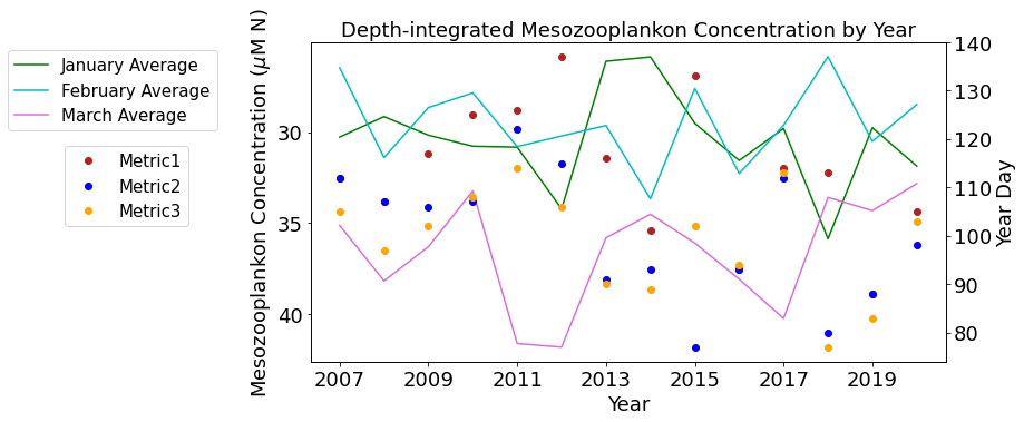
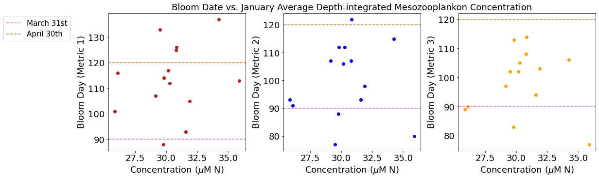
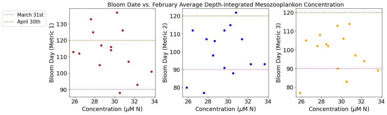
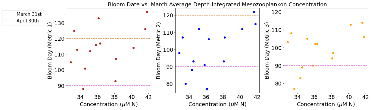
Monthly average depth-integrated microzooplankton concentration (January-March)
[21]:
fig,ax=plt.subplots(1,1,figsize=(12,5),constrained_layout=True)
p1=ax.plot(years,intmicrozoojan, '-',color='green',label='January Average')
p2=ax.plot(years,intmicrozoofeb, '-',color='c',label='February Average')
p3=ax.plot(years,intmicrozoomar, '-',color='orchid',label='March Average')
ax.set_ylabel('Microzooplankon Concentration ($\mu$M N)')
ax.set_xlabel('Year')
ax.set_title('Depth-integrated Microzooplankon Concentration by Year')
ax.set_xticks([2007,2009,2011,2013,2015,2017,2019])
ax.legend(handles=[p1[0],p2[0],p3[0]],bbox_to_anchor=(-0.49, 1.0), loc='upper left')
ax.invert_yaxis()

ax1=ax.twinx()
p4=ax1.plot(years,yearday1, 'o',color='firebrick',label='Metric1')
p5=ax1.plot(years,yearday2, 'o',color='b',label='Metric2')
p6=ax1.plot(years,yearday3, 'o',color='orange',label='Metric3')
ax1.set_ylabel('Year Day')
ax1.legend(handles=[p4[0],p5[0],p6[0]],bbox_to_anchor=(-0.4, 0.7), loc='upper left')

fig2,ax2=plt.subplots(1,3,figsize=(17,5),constrained_layout=True)
ax2[0].plot(intmicrozoojan,yearday1,'o',color='firebrick')
ax2[0].set_xlabel('Concentration ($\mu$M N)')
ax2[0].set_ylabel('Bloom Day (Metric 1)')
ax2[1].plot(intmicrozoojan,yearday2,'o',color='b')
ax2[1].set_xlabel('Concentration ($\mu$M N)')
ax2[1].set_ylabel('Bloom Day (Metric 2)')
ax2[2].plot(intmicrozoojan,yearday3,'o',color='orange')
ax2[2].set_xlabel('Concentration ($\mu$M N)')
ax2[2].set_ylabel('Bloom Day (Metric 3)')
ax2[1].set_title('Bloom Date vs. January Average Depth-integrated Microzooplankon Concentration')


fig3,ax3=plt.subplots(1,3,figsize=(17,5),constrained_layout=True)
ax3[0].plot(intmicrozoofeb,yearday1,'o',color='firebrick')
ax3[0].set_xlabel('Concentration ($\mu$M N)')
ax3[0].set_ylabel('Bloom Day (Metric 1)')
ax3[1].plot(intmicrozoofeb,yearday2,'o',color='b')
ax3[1].set_xlabel('Concentration ($\mu$M N)')
ax3[1].set_ylabel('Bloom Day (Metric 2)')
ax3[2].plot(intmicrozoofeb,yearday3,'o',color='orange')
ax3[2].set_xlabel('Concentration ($\mu$M N)')
ax3[2].set_ylabel('Bloom Day (Metric 3)')
ax3[1].set_title('Bloom Date vs. February Average Depth-integrated Microzooplankon Concentration')


fig4,ax4=plt.subplots(1,3,figsize=(17,5),constrained_layout=True)
ax4[0].plot(intmicrozoomar,yearday1,'o',color='firebrick')
ax4[0].set_xlabel('Concentration ($\mu$M N)')
ax4[0].set_ylabel('Bloom Day (Metric 1)')
ax4[1].plot(intmicrozoomar,yearday2,'o',color='b')
ax4[1].set_xlabel('Concentration ($\mu$M N)')
ax4[1].set_ylabel('Bloom Day (Metric 2)')
ax4[2].plot(intmicrozoomar,yearday3,'o',color='orange')
ax4[2].set_xlabel('Concentration ($\mu$M N)')
ax4[2].set_ylabel('Bloom Day (Metric 3)')
ax4[1].set_title('Bloom Date vs. March Average Depth-integrated Microzooplankon Concentration')


# Jan month lines
ax2[0].axhline(y=90, color='orchid', linestyle='--',label='March 31st')
ax2[0].axhline(y=120, color='peru', linestyle='--',label='April 30th')
#ax2[0].axhline(y=151, color='lime', linestyle='--',label='May 31st')
ax2[0].legend(bbox_to_anchor=(-0.25, 1.0))
ax2[1].axhline(y=90, color='orchid', linestyle='--')
ax2[2].axhline(y=90, color='orchid', linestyle='--',label='March 31st')
ax2[1].axhline(y=120, color='peru', linestyle='--')
ax2[2].axhline(y=120, color='peru', linestyle='--',label='April 30th')
# Feb month lines
ax3[0].axhline(y=90, color='orchid', linestyle='--',label='March 31st')
ax3[0].axhline(y=120, color='peru', linestyle='--',label='April 30th')
#ax3[0].axhline(y=151, color='lime', linestyle='--',label='May 31st')
ax3[0].legend(bbox_to_anchor=(-0.25, 1.0))
ax3[1].axhline(y=90, color='orchid', linestyle='--')
ax3[2].axhline(y=90, color='orchid', linestyle='--',label='March 31st')
ax3[1].axhline(y=120, color='peru', linestyle='--')
ax3[2].axhline(y=120, color='peru', linestyle='--',label='April 30th')
# March month lines
ax4[0].axhline(y=90, color='orchid', linestyle='--',label='March 31st')
ax4[0].axhline(y=120, color='peru', linestyle='--',label='April 30th')
#ax4[0].axhline(y=151, color='lime', linestyle='--',label='May 31st')
ax4[0].legend(bbox_to_anchor=(-0.25, 1.0))
ax4[1].axhline(y=90, color='orchid', linestyle='--')
ax4[2].axhline(y=90, color='orchid', linestyle='--',label='March 31st')
ax4[1].axhline(y=120, color='peru', linestyle='--')
ax4[2].axhline(y=120, color='peru', linestyle='--',label='April 30th')
[21]:
<matplotlib.lines.Line2D at 0x7f70f8ce0670>
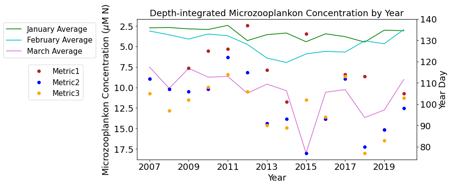
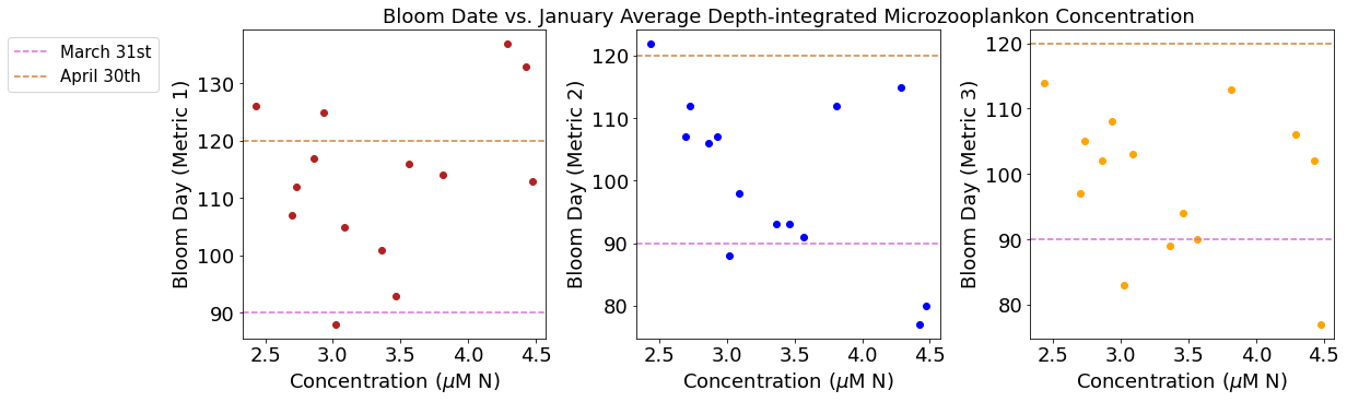
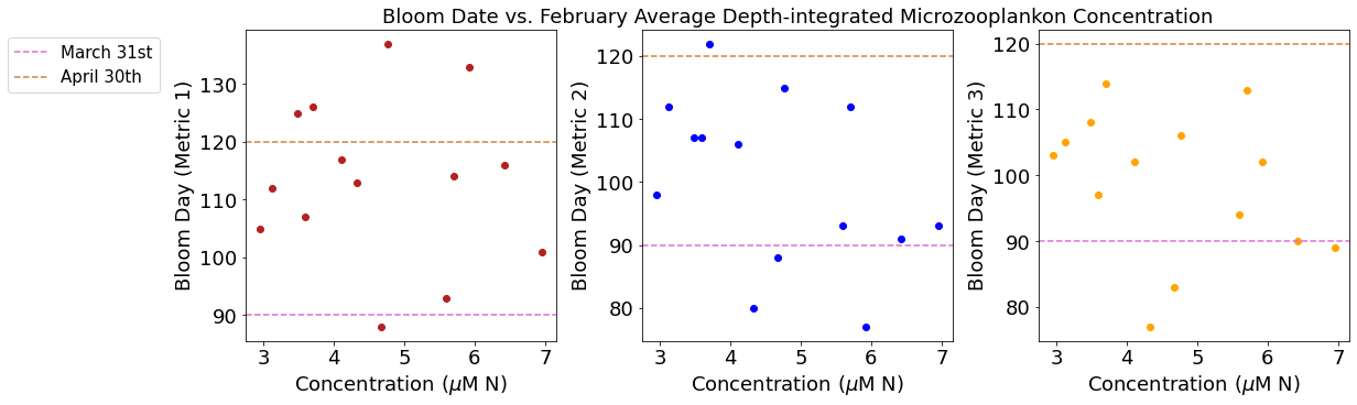
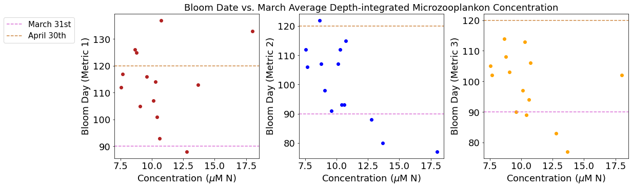
Monthly average Mid-Depth (30-90m) Nitrate (January-March)
[22]:
fig,ax=plt.subplots(1,1,figsize=(12,5),constrained_layout=True)
p1=ax.plot(years,midno3jan, '-',color='green',label='January Average')
p2=ax.plot(years,midno3feb, '-',color='c',label='February Average')
p3=ax.plot(years,midno3mar, '-',color='orchid',label='March Average')
ax.set_ylabel('Concentration ($\mu$M N)')
ax.set_xlabel('Year')
ax.set_title('Mid-depth (30-90m) Nitrate Concentration by Year')
ax.set_xticks([2007,2009,2011,2013,2015,2017,2019])
ax.legend(handles=[p1[0],p2[0],p3[0]],bbox_to_anchor=(-0.49, 1.0), loc='upper left')
ax.invert_yaxis()

ax1=ax.twinx()
p4=ax1.plot(years,yearday1, 'o',color='firebrick',label='Metric1')
p5=ax1.plot(years,yearday2, 'o',color='b',label='Metric2')
p6=ax1.plot(years,yearday3, 'o',color='orange',label='Metric3')
ax1.set_ylabel('Year Day')
ax1.legend(handles=[p4[0],p5[0],p6[0]],bbox_to_anchor=(-0.4, 0.7), loc='upper left')

#JAN
fig2,ax2=plt.subplots(1,3,figsize=(17,5),constrained_layout=True)
ax2[0].plot(midno3jan,yearday1,'o',color='firebrick')
ax2[0].set_xlabel('Concentration ($\mu$M N)')
ax2[0].set_ylabel('Bloom Day (Metric 1)')
y,r2,m,b=bloomdrivers.reg_r2(midno3jan,yearday1)
ax2[0].plot(midno3jan, y, 'r', label='Fitted line')
ax2[0].text(0.02, 0.9, '$\mathregular{r^2}$ = %.2f'%r2, transform=ax.transAxes)
ax2[0].text(0.02,0.83,f'y={round(m,1)}x+{round(b,1)}',horizontalalignment='left',verticalalignment='bottom',transform=ax.transAxes)

ax2[1].plot(midno3jan,yearday2,'o',color='b')
ax2[1].set_xlabel('Concentration ($\mu$M N)')
ax2[1].set_ylabel('Bloom Day (Metric 2)')
y,r2,m,b=bloomdrivers.reg_r2(midno3jan,yearday2)
ax2[1].plot(midno3jan, y, 'r', label='Fitted line')
ax2[1].text(0.65, 0.87, '$\mathregular{r^2}$ = %.2f'%r2, transform=ax.transAxes)
ax2[1].text(0.65,0.8,f'y={round(m,1)}x+{round(b,1)}',horizontalalignment='left',verticalalignment='bottom',transform=ax.transAxes)

ax2[2].plot(midno3jan,yearday3,'o',color='orange')
ax2[2].set_xlabel('Concentration ($\mu$M N)')
ax2[2].set_ylabel('Bloom Day (Metric 3)')
ax2[1].set_title('Bloom Date vs. January Average Mid-depth (30-90m) Nitrate Concentration')
y,r2,m,b=bloomdrivers.reg_r2(midno3jan,yearday3)
ax2[2].plot(midno3jan, y, 'r', label='Fitted line')
ax2[2].text(1.26, 0.87, '$\mathregular{r^2}$ = %.2f'%r2, transform=ax.transAxes)
ax2[2].text(1.26,0.8,f'y={round(m,1)}x+{round(b,1)}',horizontalalignment='left',verticalalignment='bottom',transform=ax.transAxes)

# FEB
fig3,ax3=plt.subplots(1,3,figsize=(17,5),constrained_layout=True)
ax3[0].plot(midno3feb,yearday1,'o',color='firebrick')
ax3[0].set_xlabel('Concentration ($\mu$M N)')
ax3[0].set_ylabel('Bloom Day (Metric 1)')
y,r2,m,b=bloomdrivers.reg_r2(midno3feb,yearday1)
ax3[0].plot(midno3feb, y, 'r', label='Fitted line')
ax3[0].text(0.02, 0.9, '$\mathregular{r^2}$ = %.2f'%r2, transform=ax.transAxes)
ax3[0].text(0.02,0.83,f'y={round(m,1)}x+{round(b,1)}',horizontalalignment='left',verticalalignment='bottom',transform=ax.transAxes)

ax3[1].plot(midno3feb,yearday2,'o',color='b')
ax3[1].set_xlabel('Concentration ($\mu$M N)')
ax3[1].set_ylabel('Bloom Day (Metric 2)')
y,r2,m,b=bloomdrivers.reg_r2(midno3feb,yearday2)
ax3[1].plot(midno3feb, y, 'r', label='Fitted line')
ax3[1].text(0.65, 0.87, '$\mathregular{r^2}$ = %.2f'%r2, transform=ax.transAxes)
ax3[1].text(0.65,0.8,f'y={round(m,1)}x+{round(b,1)}',horizontalalignment='left',verticalalignment='bottom',transform=ax.transAxes)


ax3[2].plot(midno3feb,yearday3,'o',color='orange')
ax3[2].set_xlabel('Concentration ($\mu$M N)')
ax3[2].set_ylabel('Bloom Day (Metric 3)')
ax3[1].set_title('Bloom Date vs. February Average Mid-depth (30-90m) Nitrate Concentration')
y,r2,m,b=bloomdrivers.reg_r2(midno3feb,yearday3)
ax3[2].plot(midno3feb, y, 'r', label='Fitted line')
ax3[2].text(1.26, 0.87, '$\mathregular{r^2}$ = %.2f'%r2, transform=ax.transAxes)
ax3[2].text(1.26,0.8,f'y={round(m,1)}x+{round(b,1)}',horizontalalignment='left',verticalalignment='bottom',transform=ax.transAxes)

# MAR
fig4,ax4=plt.subplots(1,3,figsize=(17,5),constrained_layout=True)
ax4[0].plot(midno3mar,yearday1,'o',color='firebrick')
ax4[0].set_xlabel('Concentration ($\mu$M N)')
ax4[0].set_ylabel('Bloom Day (Metric 1)')
y,r2,m,b=bloomdrivers.reg_r2(midno3mar,yearday1)
ax4[0].plot(midno3mar, y, 'r', label='Fitted line')
ax4[0].text(0.02, 0.9, '$\mathregular{r^2}$ = %.2f'%r2, transform=ax.transAxes)
ax4[0].text(0.02,0.83,f'y={round(m,1)}x+{round(b,1)}',horizontalalignment='left',verticalalignment='bottom',transform=ax.transAxes)

ax4[1].plot(midno3mar,yearday2,'o',color='b')
ax4[1].set_xlabel('Concentration ($\mu$M N)')
ax4[1].set_ylabel('Bloom Day (Metric 2)')
y,r2,m,b=bloomdrivers.reg_r2(midno3mar,yearday2)
ax4[1].plot(midno3mar, y, 'r', label='Fitted line')
ax4[1].text(0.65, 0.87, '$\mathregular{r^2}$ = %.2f'%r2, transform=ax.transAxes)
ax4[1].text(0.65,0.8,f'y={round(m,1)}x+{round(b,1)}',horizontalalignment='left',verticalalignment='bottom',transform=ax.transAxes)

ax4[2].plot(midno3mar,yearday3,'o',color='orange')
ax4[2].set_xlabel('Concentration ($\mu$M N)')
ax4[2].set_ylabel('Bloom Day (Metric 3)')
ax4[1].set_title('Bloom Date vs. March Average Mid-depth (30-90m) Nitrate Concentration')
y,r2,m,b=bloomdrivers.reg_r2(midno3mar,yearday3)
ax4[2].plot(midno3mar, y, 'r', label='Fitted line')
ax4[2].text(1.26, 0.87, '$\mathregular{r^2}$ = %.2f'%r2, transform=ax.transAxes)
ax4[2].text(1.26,0.8,f'y={round(m,1)}x+{round(b,1)}',horizontalalignment='left',verticalalignment='bottom',transform=ax.transAxes)

# Jan month lines
ax2[0].axhline(y=90, color='orchid', linestyle='--',label='March 31st')
ax2[0].axhline(y=120, color='peru', linestyle='--',label='April 30th')
#ax2[0].axhline(y=151, color='lime', linestyle='--',label='May 31st')
ax2[0].legend(bbox_to_anchor=(-0.25, 1.0))
ax2[1].axhline(y=90, color='orchid', linestyle='--')
ax2[2].axhline(y=90, color='orchid', linestyle='--',label='March 31st')
ax2[1].axhline(y=120, color='peru', linestyle='--')
ax2[2].axhline(y=120, color='peru', linestyle='--',label='April 30th')
# Feb month lines
ax3[0].axhline(y=90, color='orchid', linestyle='--',label='March 31st')
ax3[0].axhline(y=120, color='peru', linestyle='--',label='April 30th')
#ax3[0].axhline(y=151, color='lime', linestyle='--',label='May 31st')
ax3[0].legend(bbox_to_anchor=(-0.25, 1.0))
ax3[1].axhline(y=90, color='orchid', linestyle='--')
ax3[2].axhline(y=90, color='orchid', linestyle='--',label='March 31st')
ax3[1].axhline(y=120, color='peru', linestyle='--')
ax3[2].axhline(y=120, color='peru', linestyle='--',label='April 30th')
# March month lines
ax4[0].axhline(y=90, color='orchid', linestyle='--',label='March 31st')
ax4[0].axhline(y=120, color='peru', linestyle='--',label='April 30th')
#ax4[0].axhline(y=151, color='lime', linestyle='--',label='May 31st')
ax4[0].legend(bbox_to_anchor=(-0.25, 1.0))
ax4[1].axhline(y=90, color='orchid', linestyle='--')
ax4[2].axhline(y=90, color='orchid', linestyle='--',label='March 31st')
ax4[1].axhline(y=120, color='peru', linestyle='--')
ax4[2].axhline(y=120, color='peru', linestyle='--',label='April 30th')
[22]:
<matplotlib.lines.Line2D at 0x7f70f93af610>
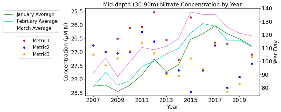
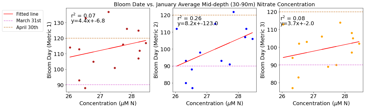
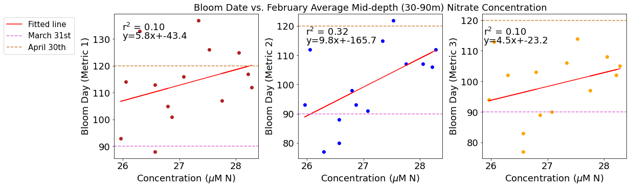
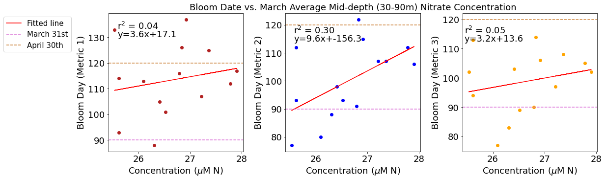
Monthly average Nitrate concentration in deep SoG (below 250 m) (January-March)
[23]:
fig,ax=plt.subplots(1,1,figsize=(12,5),constrained_layout=True)
#p1=ax.plot(years,deepno3jan, '-',color='green',label='January Average')
#p2=ax.plot(years,deepno3feb, '-',color='c',label='February Average')
p3=ax.plot(years,deepno3mar, '-',color='orchid',label='March Average')
ax.set_ylabel('Concentration ($\mu$M N)')
ax.set_xlabel('Year')
ax.set_title('Deep (below 250m) Nitrate Concentration Throughout SoG by Year')
ax.set_xticks([2007,2009,2011,2013,2015,2017,2019])
ax.legend(bbox_to_anchor=(-0.43, 1.0), loc='upper left')

ax1=ax.twinx()
p4=ax1.plot(years,yearday1, 'o',color='firebrick',label='Metric1')
p5=ax1.plot(years,yearday2, 'o',color='b',label='Metric2')
p6=ax1.plot(years,yearday3, 'o',color='orange',label='Metric3')
ax1.set_ylabel('Year Day')
ax1.legend(handles=[p4[0],p5[0],p6[0]],bbox_to_anchor=(-0.35,0.7), loc='upper left')

fig2,ax2=plt.subplots(1,3,figsize=(17,5),constrained_layout=True)
ax2[0].plot(deepno3mar,yearday1,'o',color='firebrick')
ax2[0].set_xlabel('Concentration ($\mu$M N)')
ax2[0].set_ylabel('Bloom Day (Metric 1)')
y,r2,m,b=bloomdrivers.reg_r2(deepno3mar,yearday1)
ax2[0].plot(deepno3mar, y, 'r', label='Fitted line')
ax2[0].text(0.02, 0.9, '$\mathregular{r^2}$ = %.2f'%r2, transform=ax.transAxes)
ax2[0].text(0.02,0.83,f'y={round(m,1)}x+{round(b,1)}',horizontalalignment='left',verticalalignment='bottom',transform=ax.transAxes)

ax2[1].plot(deepno3mar,yearday2,'o',color='b')
ax2[1].set_xlabel('Concentration ($\mu$M N)')
ax2[1].set_ylabel('Bloom Day (Metric 2)')
y,r2,m,b=bloomdrivers.reg_r2(deepno3mar,yearday2)
ax2[1].plot(deepno3mar, y, 'r', label='Fitted line')
ax2[1].text(0.65, 0.87, '$\mathregular{r^2}$ = %.2f'%r2, transform=ax.transAxes)
ax2[1].text(0.65,0.8,f'y={round(m,1)}x+{round(b,1)}',horizontalalignment='left',verticalalignment='bottom',transform=ax.transAxes)

ax2[2].plot(deepno3mar,yearday3,'o',color='orange')
ax2[2].set_xlabel('Concentration ($\mu$M N)')
ax2[2].set_ylabel('Bloom Day (Metric 3)')
y,r2,m,b=bloomdrivers.reg_r2(deepno3mar,yearday3)
ax2[2].plot(deepno3mar, y, 'r', label='Fitted line')
ax2[2].text(1.26, 0.87, '$\mathregular{r^2}$ = %.2f'%r2, transform=ax.transAxes)
ax2[2].text(1.26,0.8,f'y={round(m,1)}x+{round(b,1)}',horizontalalignment='left',verticalalignment='bottom',transform=ax.transAxes)
ax2[1].set_title('Bloom Date vs. January Average Deep (below 250m) Nitrate Concentration Throughout SoG')

# Jan month lines
ax2[0].axhline(y=90, color='orchid', linestyle='--',label='March 31st')
ax2[0].axhline(y=120, color='peru', linestyle='--',label='April 30th')
#ax2[0].axhline(y=151, color='lime', linestyle='--',label='May 31st')
ax2[0].legend(bbox_to_anchor=(-0.25, 1.0))
ax2[1].axhline(y=90, color='orchid', linestyle='--')
ax2[2].axhline(y=90, color='orchid', linestyle='--',label='March 31st')
ax2[1].axhline(y=120, color='peru', linestyle='--')
ax2[2].axhline(y=120, color='peru', linestyle='--',label='April 30th')
[23]:
<matplotlib.lines.Line2D at 0x7f70f92bc9d0>
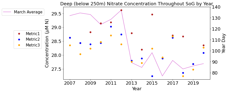
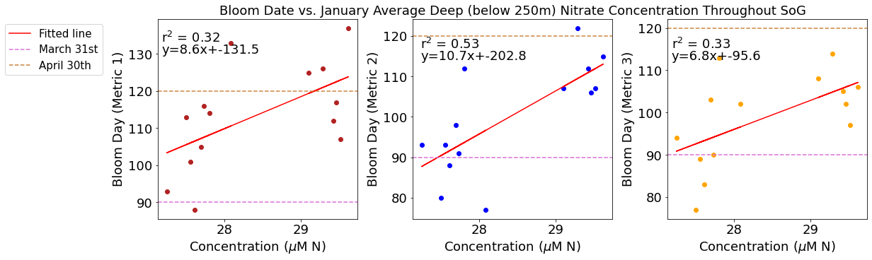
Monthly Average Halocline Depth (January-March)
[24]:
fig,ax=plt.subplots(1,1,figsize=(12,5),constrained_layout=True)
p1=ax.plot(years,halojan, '-',color='green',label='January Average')
p2=ax.plot(years,halofeb, '-',color='c',label='February Average')
p3=ax.plot(years,halomar, '-',color='orchid',label='March Average')
ax.set_ylabel('Halocline Depth (m)')
ax.set_xlabel('Year')
ax.set_title('Halocline Depth by Year')
ax.set_xticks([2007,2009,2011,2013,2015,2017,2019])
ax.legend(handles=[p1[0],p2[0],p3[0]],bbox_to_anchor=(-0.45, 1.0), loc='upper left')
ax.invert_yaxis()

ax1=ax.twinx()
p4=ax1.plot(years,yearday1, 'o',color='firebrick',label='Metric1')
p5=ax1.plot(years,yearday2, 'o',color='b',label='Metric2')
p6=ax1.plot(years,yearday3, 'o',color='orange',label='Metric3')
ax1.set_ylabel('Year Day')
ax1.legend(handles=[p4[0],p5[0],p6[0]],bbox_to_anchor=(-0.38, 0.7), loc='upper left')

# JAN
fig2,ax2=plt.subplots(1,3,figsize=(17,5),constrained_layout=True)
ax2[0].plot(halojan,yearday1,'o',color='firebrick')
ax2[0].set_xlabel('Halocline Depth (m)')
ax2[0].set_ylabel('Bloom Day (Metric 1)')
y,r2,m,b=bloomdrivers.reg_r2(halojan,yearday1)
ax2[0].plot(halojan, y, 'r', label='Fitted line')
ax2[0].text(0.02, 0.9, '$\mathregular{r^2}$ = %.2f'%r2, transform=ax.transAxes)
ax2[0].text(0.02,0.83,f'y={round(m,1)}x+{round(b,1)}',horizontalalignment='left',verticalalignment='bottom',transform=ax.transAxes)

ax2[1].plot(halojan,yearday2,'o',color='b')
ax2[1].set_xlabel('Halocline Depth (m)')
ax2[1].set_ylabel('Bloom Day (Metric 2)')
y,r2,m,b=bloomdrivers.reg_r2(halojan,yearday2)
ax2[1].plot(halojan, y, 'r', label='Fitted line')
ax2[1].text(0.65, 0.87, '$\mathregular{r^2}$ = %.2f'%r2, transform=ax.transAxes)
ax2[1].text(0.65,0.8,f'y={round(m,1)}x+{round(b,1)}',horizontalalignment='left',verticalalignment='bottom',transform=ax.transAxes)

ax2[2].plot(halojan,yearday3,'o',color='orange')
ax2[2].set_xlabel('Halocline Depth (m)')
ax2[2].set_ylabel('Bloom Day (Metric 3)')
ax2[1].set_title('Bloom Date vs. January Average Halocline Depth')
y,r2,m,b=bloomdrivers.reg_r2(halojan,yearday3)
ax2[2].plot(halojan, y, 'r', label='Fitted line')
ax2[2].text(1.26, 0.87, '$\mathregular{r^2}$ = %.2f'%r2, transform=ax.transAxes)
ax2[2].text(1.26,0.8,f'y={round(m,1)}x+{round(b,1)}',horizontalalignment='left',verticalalignment='bottom',transform=ax.transAxes)

# FEB
fig3,ax3=plt.subplots(1,3,figsize=(17,5),constrained_layout=True)
ax3[0].plot(halofeb,yearday1,'o',color='firebrick')
ax3[0].set_xlabel('Halocline Depth (m)')
ax3[0].set_ylabel('Bloom Day (Metric 1)')
y,r2,m,b=bloomdrivers.reg_r2(halofeb,yearday1)
ax3[0].plot(halofeb, y, 'r', label='Fitted line')
ax3[0].text(0.02, 0.9, '$\mathregular{r^2}$ = %.2f'%r2, transform=ax.transAxes)
ax3[0].text(0.02,0.83,f'y={round(m,1)}x+{round(b,1)}',horizontalalignment='left',verticalalignment='bottom',transform=ax.transAxes)

ax3[1].plot(halofeb,yearday2,'o',color='b')
ax3[1].set_xlabel('Halocline Depth (m)')
ax3[1].set_ylabel('Bloom Day (Metric 2)')
y,r2,m,b=bloomdrivers.reg_r2(halofeb,yearday2)
ax3[1].plot(halofeb, y, 'r', label='Fitted line')
ax3[1].text(0.65, 0.87, '$\mathregular{r^2}$ = %.2f'%r2, transform=ax.transAxes)
ax3[1].text(0.65,0.8,f'y={round(m,1)}x+{round(b,1)}',horizontalalignment='left',verticalalignment='bottom',transform=ax.transAxes)

ax3[2].plot(halofeb,yearday3,'o',color='orange')
ax3[2].set_xlabel('Halocline Depth (m)')
ax3[2].set_ylabel('Bloom Day (Metric 3)')
ax3[1].set_title('Bloom Date vs. February Average Halocline Depth')
y,r2,m,b=bloomdrivers.reg_r2(halofeb,yearday3)
ax3[2].plot(halofeb, y, 'r', label='Fitted line')
ax3[2].text(1.26, 0.87, '$\mathregular{r^2}$ = %.2f'%r2, transform=ax.transAxes)
ax3[2].text(1.26,0.8,f'y={round(m,1)}x+{round(b,1)}',horizontalalignment='left',verticalalignment='bottom',transform=ax.transAxes)

# MAR
fig4,ax4=plt.subplots(1,3,figsize=(17,5),constrained_layout=True)
ax4[0].plot(halomar,yearday1,'o',color='firebrick')
ax4[0].set_xlabel('Halocline Depth (m)')
ax4[0].set_ylabel('Bloom Day (Metric 1)')
y,r2,m,b=bloomdrivers.reg_r2(halomar,yearday1)
ax4[0].plot(halomar, y, 'r', label='Fitted line')
ax4[0].text(0.02, 0.9, '$\mathregular{r^2}$ = %.2f'%r2, transform=ax.transAxes)
ax4[0].text(0.02,0.83,f'y={round(m,1)}x+{round(b,1)}',horizontalalignment='left',verticalalignment='bottom',transform=ax.transAxes)

ax4[1].plot(halomar,yearday2,'o',color='b')
ax4[1].set_xlabel('Halocline Depth (m)')
ax4[1].set_ylabel('Bloom Day (Metric 2)')
y,r2,m,b=bloomdrivers.reg_r2(halomar,yearday2)
ax4[1].plot(halomar, y, 'r', label='Fitted line')
ax4[1].text(0.65, 0.87, '$\mathregular{r^2}$ = %.2f'%r2, transform=ax.transAxes)
ax4[1].text(0.65,0.8,f'y={round(m,1)}x+{round(b,1)}',horizontalalignment='left',verticalalignment='bottom',transform=ax.transAxes)

ax4[2].plot(halomar,yearday3,'o',color='orange')
ax4[2].set_xlabel('Halocline Depth (m)')
ax4[2].set_ylabel('Bloom Day (Metric 3)')
ax4[1].set_title('Bloom Date vs. March Average Halocline Depth')
y,r2,m,b=bloomdrivers.reg_r2(halomar,yearday3)
ax4[2].plot(halomar, y, 'r', label='Fitted line')
ax4[2].text(1.26, 0.87, '$\mathregular{r^2}$ = %.2f'%r2, transform=ax.transAxes)
ax4[2].text(1.26,0.8,f'y={round(m,1)}x+{round(b,1)}',horizontalalignment='left',verticalalignment='bottom',transform=ax.transAxes)


# Jan month lines
ax2[0].axhline(y=90, color='orchid', linestyle='--',label='March 31st')
ax2[0].axhline(y=120, color='peru', linestyle='--',label='April 30th')
#ax2[0].axhline(y=151, color='lime', linestyle='--',label='May 31st')
ax2[0].legend(bbox_to_anchor=(-0.25, 1.0))
ax2[1].axhline(y=90, color='orchid', linestyle='--')
ax2[2].axhline(y=90, color='orchid', linestyle='--',label='March 31st')
ax2[1].axhline(y=120, color='peru', linestyle='--')
ax2[2].axhline(y=120, color='peru', linestyle='--',label='April 30th')
# Feb month lines
ax3[0].axhline(y=90, color='orchid', linestyle='--',label='March 31st')
ax3[0].axhline(y=120, color='peru', linestyle='--',label='April 30th')
#ax3[0].axhline(y=151, color='lime', linestyle='--',label='May 31st')
ax3[0].legend(bbox_to_anchor=(-0.25, 1.0))
ax3[1].axhline(y=90, color='orchid', linestyle='--')
ax3[2].axhline(y=90, color='orchid', linestyle='--',label='March 31st')
ax3[1].axhline(y=120, color='peru', linestyle='--')
ax3[2].axhline(y=120, color='peru', linestyle='--',label='April 30th')
# March month lines
ax4[0].axhline(y=90, color='orchid', linestyle='--',label='March 31st')
ax4[0].axhline(y=120, color='peru', linestyle='--',label='April 30th')
#ax4[0].axhline(y=151, color='lime', linestyle='--',label='May 31st')
ax4[0].legend(bbox_to_anchor=(-0.25, 1.0))
ax4[1].axhline(y=90, color='orchid', linestyle='--')
ax4[2].axhline(y=90, color='orchid', linestyle='--',label='March 31st')
ax4[1].axhline(y=120, color='peru', linestyle='--')
ax4[2].axhline(y=120, color='peru', linestyle='--',label='April 30th')
[24]:
<matplotlib.lines.Line2D at 0x7f70f934b940>
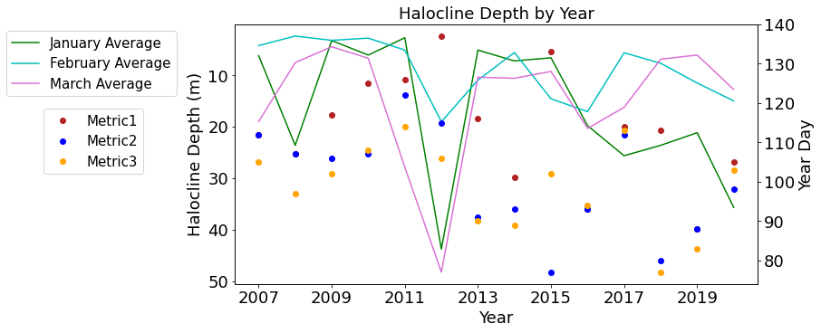
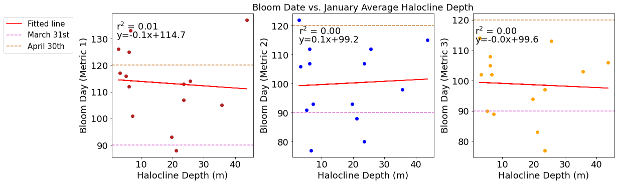
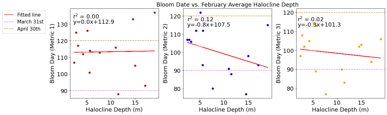
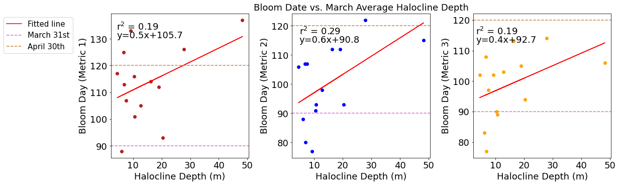
Monthly average turbocline depth (January-March)
[25]:
fig,ax=plt.subplots(1,1,figsize=(12,5),constrained_layout=True)
p1=ax.plot(years,turbojan, '-',color='green',label='January Average')
p2=ax.plot(years,turbofeb, '-',color='c',label='February Average')
p3=ax.plot(years,turbomar, '-',color='orchid',label='March Average')
ax.set_ylabel('Turbocline Depth (m)')
ax.set_xlabel('Year')
ax.set_title('Turbocline Depth by Year')
ax.set_xticks([2007,2009,2011,2013,2015,2017,2019])
ax.legend(handles=[p1[0],p2[0],p3[0]],bbox_to_anchor=(-0.45, 1.0), loc='upper left')

ax1=ax.twinx()
p4=ax1.plot(years,yearday1, 'o',color='firebrick',label='Metric1')
p5=ax1.plot(years,yearday2, 'o',color='b',label='Metric2')
p6=ax1.plot(years,yearday3, 'o',color='orange',label='Metric3')
ax1.set_ylabel('Year Day')
ax1.legend(handles=[p4[0],p5[0],p6[0]],bbox_to_anchor=(-0.38, 0.7), loc='upper left')

# ---------- Jan ---------
fig2,ax2=plt.subplots(1,3,figsize=(17,5),constrained_layout=True)
ax2[0].plot(turbojan,yearday1,'o',color='firebrick')
ax2[0].set_xlabel('Turbocline Depth (m)')
ax2[0].set_ylabel('Bloom Day (Metric 1)')
y,r2,m,b=bloomdrivers.reg_r2(turbojan,yearday1)
ax2[0].plot(turbojan, y, 'r', label='Fitted Line')
ax2[0].text(0.02, 0.9, '$\mathregular{r^2}$ = %.2f'%r2, transform=ax.transAxes)
ax2[0].text(0.02,0.83,f'y={round(m,1)}x+{round(b,1)}',horizontalalignment='left',verticalalignment='bottom',transform=ax.transAxes)

ax2[1].plot(turbojan,yearday2,'o',color='b')
ax2[1].set_xlabel('Turbocline Depth (m)')
ax2[1].set_ylabel('Bloom Day (Metric 2)')
y,r2,m,b=bloomdrivers.reg_r2(turbojan,yearday2)
ax2[1].plot(turbojan, y, 'r', label='Fitted line')
ax2[1].text(0.65, 0.87, '$\mathregular{r^2}$ = %.2f'%r2, transform=ax.transAxes)
ax2[1].text(0.65,0.8,f'y={round(m,1)}x+{round(b,1)}',horizontalalignment='left',verticalalignment='bottom',transform=ax.transAxes)

ax2[2].plot(turbojan,yearday3,'o',color='orange')
ax2[2].set_xlabel('Turbocline Depth (m)')
ax2[2].set_ylabel('Bloom Day (Metric 3)')
y,r2,m,b=bloomdrivers.reg_r2(turbojan,yearday3)
ax2[2].plot(turbojan, y, 'r', label='Fitted line')
ax2[2].text(1.26, 0.87, '$\mathregular{r^2}$ = %.2f'%r2, transform=ax.transAxes)
ax2[2].text(1.26,0.8,f'y={round(m,1)}x+{round(b,1)}',horizontalalignment='left',verticalalignment='bottom',transform=ax.transAxes)

ax2[1].set_title('Bloom Date vs. January Average Turbocline Depth')

# ---------- Feb ---------
fig3,ax3=plt.subplots(1,3,figsize=(17,5),constrained_layout=True)
ax3[0].plot(turbofeb,yearday1,'o',color='firebrick')
ax3[0].set_xlabel('Turbocline Depth (m)')
ax3[0].set_ylabel('Bloom Day (Metric 1)')
y,r2,m,b=bloomdrivers.reg_r2(turbofeb,yearday1)
ax3[0].plot(turbofeb, y, 'r', label='Fitted line')
ax3[0].text(0.02, 0.9, '$\mathregular{r^2}$ = %.2f'%r2, transform=ax.transAxes)
ax3[0].text(0.02,0.83,f'y={round(m,1)}x+{round(b,1)}',horizontalalignment='left',verticalalignment='bottom',transform=ax.transAxes)

ax3[1].plot(turbofeb,yearday2,'o',color='b')
ax3[1].set_xlabel('Turbocline Depth (m)')
ax3[1].set_ylabel('Bloom Day (Metric 2)')
y,r2,m,b=bloomdrivers.reg_r2(turbofeb,yearday2)
ax3[1].plot(turbofeb, y, 'r', label='Fitted line')
ax3[1].text(0.65, 0.87, '$\mathregular{r^2}$ = %.2f'%r2, transform=ax.transAxes)
ax3[1].text(0.65,0.8,f'y={round(m,1)}x+{round(b,1)}',horizontalalignment='left',verticalalignment='bottom',transform=ax.transAxes)

ax3[2].plot(turbofeb,yearday3,'o',color='orange')
ax3[2].set_xlabel('Turbocline Depth (m)')
ax3[2].set_ylabel('Bloom Day (Metric 3)')
y,r2,m,b=bloomdrivers.reg_r2(turbofeb,yearday3)
ax3[2].plot(turbofeb, y, 'r', label='Fitted line')
ax3[2].text(1.26, 0.87, '$\mathregular{r^2}$ = %.2f'%r2, transform=ax.transAxes)
ax3[2].text(1.26,0.8,f'y={round(m,1)}x+{round(b,1)}',horizontalalignment='left',verticalalignment='bottom',transform=ax.transAxes)

ax3[1].set_title('Bloom Date vs. February Average Turbocline Depth')

# ---------- March ---------
fig4,ax4=plt.subplots(1,3,figsize=(17,5),constrained_layout=True)
ax4[0].plot(turbomar,yearday1,'o',color='firebrick')
ax4[0].set_xlabel('Turbocline Depth (m)')
ax4[0].set_ylabel('Bloom Day (Metric 1)')
y,r2,m,b=bloomdrivers.reg_r2(turbomar,yearday1)
ax4[0].plot(turbomar, y, 'r', label='Fitted line')
ax4[0].text(0.02, 0.9, '$\mathregular{r^2}$ = %.2f'%r2, transform=ax.transAxes)
ax4[0].text(0.02,0.83,f'y={round(m,1)}x+{round(b,1)}',horizontalalignment='left',verticalalignment='bottom',transform=ax.transAxes)

ax4[1].plot(turbomar,yearday2,'o',color='b')
ax4[1].set_xlabel('Turbocline Depth (m)')
ax4[1].set_ylabel('Bloom Day (Metric 2)')
ax4[1].set_title('Bloom Date vs. March Average Turbocline Depth')
y,r2,m,b=bloomdrivers.reg_r2(turbomar,yearday2)
ax4[1].plot(turbomar, y, 'r', label='Fitted line')
ax4[1].text(0.65, 0.87, '$\mathregular{r^2}$ = %.2f'%r2, transform=ax.transAxes)
ax4[1].text(0.65,0.8,f'y={round(m,1)}x+{round(b,1)}',horizontalalignment='left',verticalalignment='bottom',transform=ax.transAxes)

ax4[2].plot(turbomar,yearday3,'o',color='orange')
ax4[2].set_xlabel('Turbocline Depth (m)')
ax4[2].set_ylabel('Bloom Day (Metric 3)')
y,r2,m,b=bloomdrivers.reg_r2(turbomar,yearday3)
ax4[2].plot(turbomar, y, 'r', label='Fitted line')
ax4[2].text(1.26, 0.87, '$\mathregular{r^2}$ = %.2f'%r2, transform=ax.transAxes)
ax4[2].text(1.26,0.8,f'y={round(m,1)}x+{round(b,1)}',horizontalalignment='left',verticalalignment='bottom',transform=ax.transAxes)

# Jan month lines
ax2[0].axhline(y=90, color='orchid', linestyle='--',label='March 31st')
ax2[0].axhline(y=120, color='peru', linestyle='--',label='April 30th')
ax2[0].legend(bbox_to_anchor=(-0.25, 1.0))
ax2[1].axhline(y=90, color='orchid', linestyle='--')
ax2[2].axhline(y=90, color='orchid', linestyle='--',label='March 31st')
ax2[1].axhline(y=120, color='peru', linestyle='--')
ax2[2].axhline(y=120, color='peru', linestyle='--',label='April 30th')
# Feb month lines
ax3[0].axhline(y=90, color='orchid', linestyle='--',label='March 31st')
ax3[0].axhline(y=120, color='peru', linestyle='--',label='April 30th')
ax3[0].legend(bbox_to_anchor=(-0.25, 1.0))
ax3[1].axhline(y=90, color='orchid', linestyle='--')
ax3[2].axhline(y=90, color='orchid', linestyle='--',label='March 31st')
ax3[1].axhline(y=120, color='peru', linestyle='--')
ax3[2].axhline(y=120, color='peru', linestyle='--',label='April 30th')
# March month lines
ax4[0].axhline(y=90, color='orchid', linestyle='--',label='March 31st')
ax4[0].axhline(y=120, color='peru', linestyle='--',label='April 30th')
ax4[0].legend(bbox_to_anchor=(-0.25, 1.0))
ax4[1].axhline(y=90, color='orchid', linestyle='--')
ax4[2].axhline(y=90, color='orchid', linestyle='--',label='March 31st')
ax4[1].axhline(y=120, color='peru', linestyle='--')
ax4[2].axhline(y=120, color='peru', linestyle='--',label='April 30th')
[25]:
<matplotlib.lines.Line2D at 0x7f70f8d5da00>
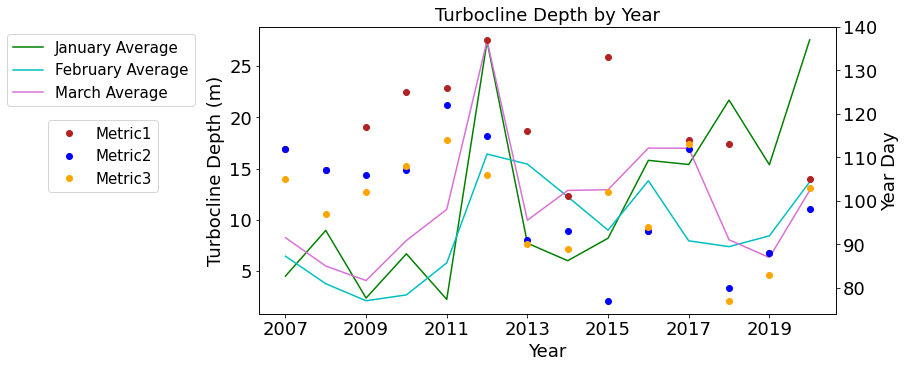
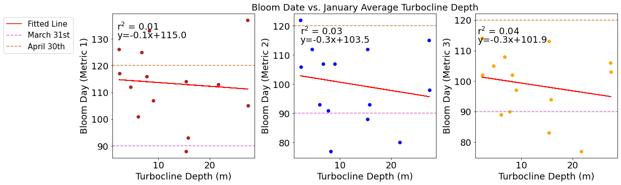
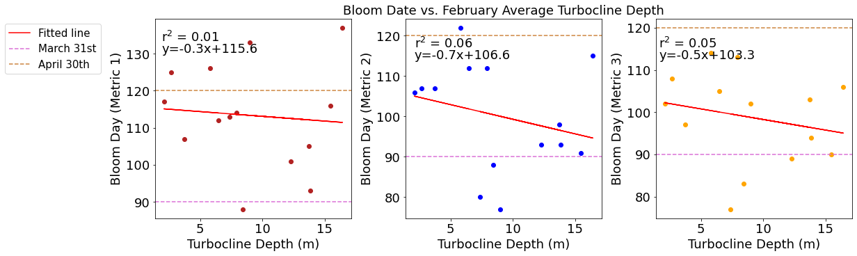
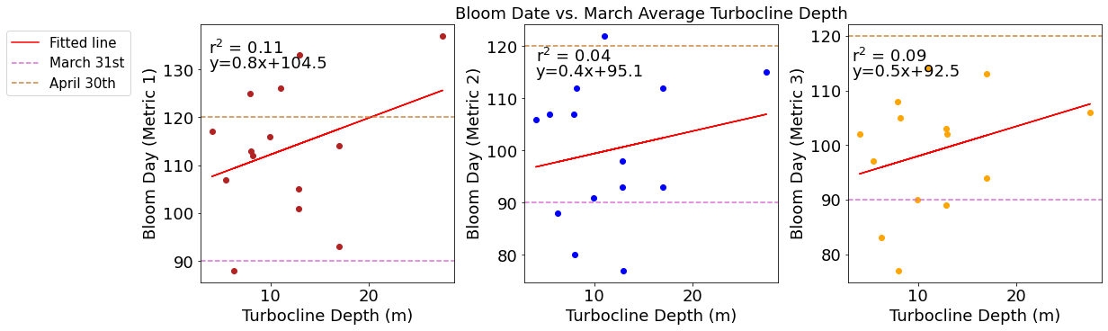
Monthly average density difference from surface to 10m (January-March)
[26]:
fig,ax=plt.subplots(1,1,figsize=(12,5),constrained_layout=True)
p1=ax.plot(years,densdiff10jan, '-',color='green',label='January Average')
p2=ax.plot(years,densdiff10feb, '-',color='c',label='February Average')
p3=ax.plot(years,densdiff10mar, '-',color='orchid',label='March Average')
ax.set_ylabel('Density (kg/$\mathregular{m^3}$)')
ax.set_xlabel('Year')
ax.set_title('Density difference from surface to 10m by Year')
ax.set_xticks([2007,2009,2011,2013,2015,2017,2019])
ax.legend(handles=[p1[0],p2[0],p3[0]],bbox_to_anchor=(-0.45, 1.0), loc='upper left')

ax1=ax.twinx()
p4=ax1.plot(years,yearday1, 'o',color='firebrick',label='Metric1')
p5=ax1.plot(years,yearday2, 'o',color='b',label='Metric2')
p6=ax1.plot(years,yearday3, 'o',color='orange',label='Metric3')
ax1.set_ylabel('Year Day')
ax1.legend(handles=[p4[0],p5[0],p6[0]],bbox_to_anchor=(-0.38, 0.7), loc='upper left')

# ---------- Jan ---------
fig2,ax2=plt.subplots(1,3,figsize=(17,5),constrained_layout=True)
ax2[0].plot(densdiff10jan,yearday1,'o',color='firebrick')
ax2[0].set_xlabel('Density (kg/$\mathregular{m^3}$)')
ax2[0].set_ylabel('Bloom Day (Metric 1)')
y,r2,m,b=bloomdrivers.reg_r2(densdiff10jan,yearday1)
ax2[0].plot(densdiff10jan, y, 'r', label='Fitted Line')
ax2[0].text(0.02, 0.9, '$\mathregular{r^2}$ = %.2f'%r2, transform=ax.transAxes)
ax2[0].text(0.02,0.83,f'y={round(m,1)}x+{round(b,1)}',horizontalalignment='left',verticalalignment='bottom',transform=ax.transAxes)

ax2[1].plot(densdiff10jan,yearday2,'o',color='b')
ax2[1].set_xlabel('Density (kg/$\mathregular{m^3}$)')
ax2[1].set_ylabel('Bloom Day (Metric 2)')
y,r2,m,b=bloomdrivers.reg_r2(densdiff10jan,yearday2)
ax2[1].plot(densdiff10jan, y, 'r', label='Fitted line')
ax2[1].text(0.65, 0.87, '$\mathregular{r^2}$ = %.2f'%r2, transform=ax.transAxes)
ax2[1].text(0.65,0.8,f'y={round(m,1)}x+{round(b,1)}',horizontalalignment='left',verticalalignment='bottom',transform=ax.transAxes)

ax2[2].plot(densdiff10jan,yearday3,'o',color='orange')
ax2[2].set_xlabel('Density (kg/$\mathregular{m^3}$)')
ax2[2].set_ylabel('Bloom Day (Metric 3)')
y,r2,m,b=bloomdrivers.reg_r2(densdiff10jan,yearday3)
ax2[2].plot(densdiff10jan, y, 'r', label='Fitted line')
ax2[2].text(1.26, 0.87, '$\mathregular{r^2}$ = %.2f'%r2, transform=ax.transAxes)
ax2[2].text(1.26,0.8,f'y={round(m,1)}x+{round(b,1)}',horizontalalignment='left',verticalalignment='bottom',transform=ax.transAxes)

ax2[1].set_title('Bloom Date vs. January Average Density Difference from Surface to 10m')

# ---------- Feb ---------
fig3,ax3=plt.subplots(1,3,figsize=(17,5),constrained_layout=True)
ax3[0].plot(densdiff10feb,yearday1,'o',color='firebrick')
ax3[0].set_xlabel('Density (kg/$\mathregular{m^3}$)')
ax3[0].set_ylabel('Bloom Day (Metric 1)')
y,r2,m,b=bloomdrivers.reg_r2(densdiff10feb,yearday1)
ax3[0].plot(densdiff10feb, y, 'r', label='Fitted line')
ax3[0].text(0.02, 0.9, '$\mathregular{r^2}$ = %.2f'%r2, transform=ax.transAxes)
ax3[0].text(0.02,0.83,f'y={round(m,1)}x+{round(b,1)}',horizontalalignment='left',verticalalignment='bottom',transform=ax.transAxes)

ax3[1].plot(densdiff10feb,yearday2,'o',color='b')
ax3[1].set_xlabel('Density (kg/$\mathregular{m^3}$)')
ax3[1].set_ylabel('Bloom Day (Metric 2)')
y,r2,m,b=bloomdrivers.reg_r2(densdiff10feb,yearday2)
ax3[1].plot(densdiff10feb, y, 'r', label='Fitted line')
ax3[1].text(0.65, 0.87, '$\mathregular{r^2}$ = %.2f'%r2, transform=ax.transAxes)
ax3[1].text(0.65,0.8,f'y={round(m,1)}x+{round(b,1)}',horizontalalignment='left',verticalalignment='bottom',transform=ax.transAxes)

ax3[2].plot(densdiff10feb,yearday3,'o',color='orange')
ax3[2].set_xlabel('Density (kg/$\mathregular{m^3}$)')
ax3[2].set_ylabel('Bloom Day (Metric 3)')
y,r2,m,b=bloomdrivers.reg_r2(densdiff10feb,yearday3)
ax3[2].plot(densdiff10feb, y, 'r', label='Fitted line')
ax3[2].text(1.26, 0.87, '$\mathregular{r^2}$ = %.2f'%r2, transform=ax.transAxes)
ax3[2].text(1.26,0.8,f'y={round(m,1)}x+{round(b,1)}',horizontalalignment='left',verticalalignment='bottom',transform=ax.transAxes)

ax3[1].set_title('Bloom Date vs. February Average Density Difference from Surface to 10m')

# ---------- March ---------
fig4,ax4=plt.subplots(1,3,figsize=(17,5),constrained_layout=True)
ax4[0].plot(densdiff10mar,yearday1,'o',color='firebrick')
ax4[0].set_xlabel('Density (kg/$\mathregular{m^3}$)')
ax4[0].set_ylabel('Bloom Day (Metric 1)')
y,r2,m,b=bloomdrivers.reg_r2(densdiff10mar,yearday1)
ax4[0].plot(densdiff10mar, y, 'r', label='Fitted line')
ax4[0].text(0.02, 0.9, '$\mathregular{r^2}$ = %.2f'%r2, transform=ax.transAxes)
ax4[0].text(0.02,0.83,f'y={round(m,1)}x+{round(b,1)}',horizontalalignment='left',verticalalignment='bottom',transform=ax.transAxes)

ax4[1].plot(densdiff10mar,yearday2,'o',color='b')
ax4[1].set_xlabel('Density (kg/$\mathregular{m^3}$)')
ax4[1].set_ylabel('Bloom Day (Metric 2)')
y,r2,m,b=bloomdrivers.reg_r2(densdiff10mar,yearday2)
ax4[1].plot(densdiff10mar, y, 'r', label='Fitted line')
ax4[1].text(0.65, 0.87, '$\mathregular{r^2}$ = %.2f'%r2, transform=ax.transAxes)
ax4[1].text(0.65,0.8,f'y={round(m,1)}x+{round(b,1)}',horizontalalignment='left',verticalalignment='bottom',transform=ax.transAxes)

ax4[2].plot(densdiff10mar,yearday3,'o',color='orange')
ax4[2].set_xlabel('Density (kg/$\mathregular{m^3}$)')
ax4[2].set_ylabel('Bloom Day (Metric 3)')
y,r2,m,b=bloomdrivers.reg_r2(densdiff10mar,yearday3)
ax4[2].plot(densdiff10mar, y, 'r', label='Fitted line')
ax4[2].text(1.26, 0.87, '$\mathregular{r^2}$ = %.2f'%r2, transform=ax.transAxes)
ax4[2].text(1.26,0.8,f'y={round(m,1)}x+{round(b,1)}',horizontalalignment='left',verticalalignment='bottom',transform=ax.transAxes)

ax4[1].set_title('Bloom Date vs. March Average Density Difference from Surface to 10m')

# Jan month lines
ax2[0].axhline(y=90, color='orchid', linestyle='--',label='March 31st')
ax2[0].axhline(y=120, color='peru', linestyle='--',label='April 30th')
ax2[0].legend(bbox_to_anchor=(-0.25, 1.0))
ax2[1].axhline(y=90, color='orchid', linestyle='--')
ax2[2].axhline(y=90, color='orchid', linestyle='--',label='March 31st')
ax2[1].axhline(y=120, color='peru', linestyle='--')
ax2[2].axhline(y=120, color='peru', linestyle='--',label='April 30th')
# Feb month lines
ax3[0].axhline(y=90, color='orchid', linestyle='--',label='March 31st')
ax3[0].axhline(y=120, color='peru', linestyle='--',label='April 30th')
ax3[0].legend(bbox_to_anchor=(-0.25, 1.0))
ax3[1].axhline(y=90, color='orchid', linestyle='--')
ax3[2].axhline(y=90, color='orchid', linestyle='--',label='March 31st')
ax3[1].axhline(y=120, color='peru', linestyle='--')
ax3[2].axhline(y=120, color='peru', linestyle='--',label='April 30th')
# March month lines
ax4[0].axhline(y=90, color='orchid', linestyle='--',label='March 31st')
ax4[0].axhline(y=120, color='peru', linestyle='--',label='April 30th')
ax4[0].legend(bbox_to_anchor=(-0.25, 1.0))
ax4[1].axhline(y=90, color='orchid', linestyle='--')
ax4[2].axhline(y=90, color='orchid', linestyle='--',label='March 31st')
ax4[1].axhline(y=120, color='peru', linestyle='--')
ax4[2].axhline(y=120, color='peru', linestyle='--',label='April 30th')
[26]:
<matplotlib.lines.Line2D at 0x7f70f8ca2280>
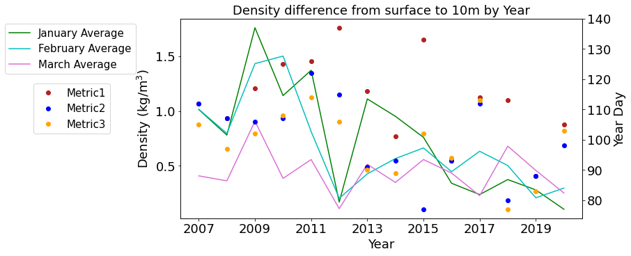
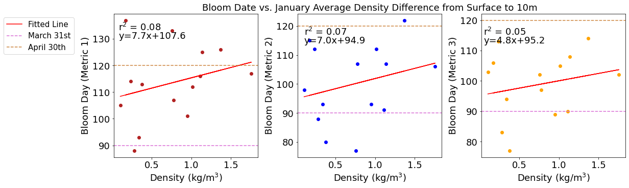
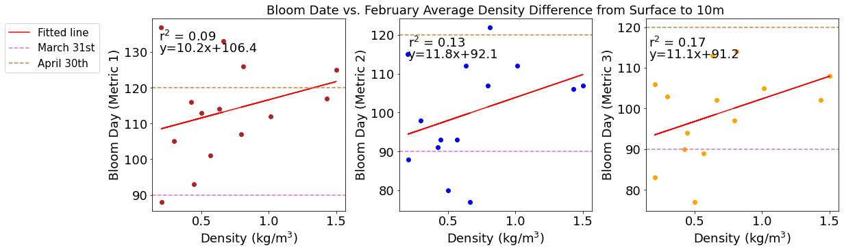
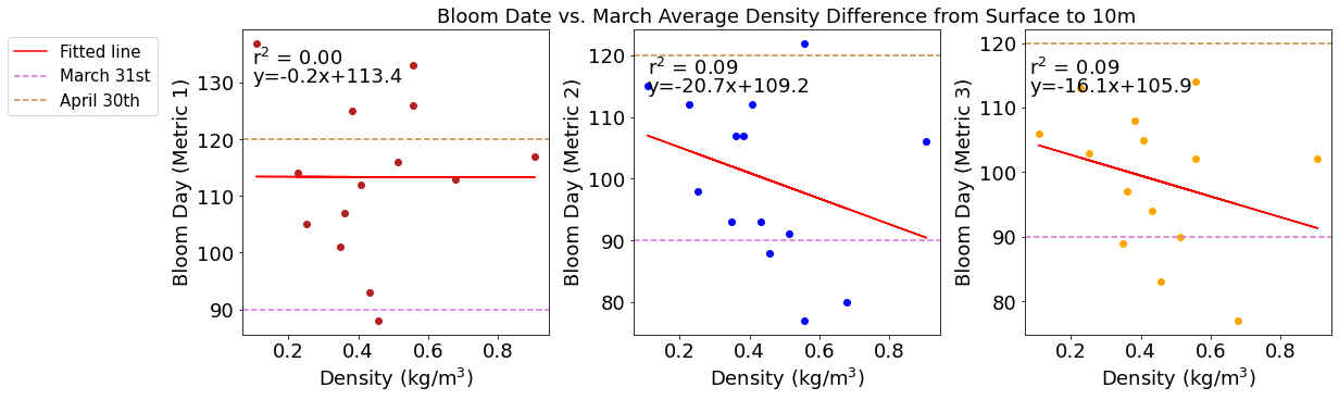
Monthly average eddy diffusivity in top 15m (January-March)
[27]:
fig,ax=plt.subplots(1,1,figsize=(12,5),constrained_layout=True)
p1=ax.plot(years,eddy15jan, '-',color='green',label='January Average')
p2=ax.plot(years,eddy15feb, '-',color='c',label='February Average')
p3=ax.plot(years,eddy15mar, '-',color='orchid',label='March Average')
ax.set_ylabel('Eddy Diffusivity ($\mathregular{m^2}$/s)')
ax.set_xlabel('Year')
ax.set_title('Average Eddy Diffusivity from Surface to 15m by Year')
ax.set_xticks([2007,2009,2011,2013,2015,2017,2019])
ax.legend(handles=[p1[0],p2[0],p3[0]],bbox_to_anchor=(-0.5, 1.0), loc='upper left')

ax1=ax.twinx()
p4=ax1.plot(years,yearday1, 'o',color='firebrick',label='Metric1')
p5=ax1.plot(years,yearday2, 'o',color='b',label='Metric2')
p6=ax1.plot(years,yearday3, 'o',color='orange',label='Metric3')
ax1.set_ylabel('Year Day')
ax1.legend(handles=[p4[0],p5[0],p6[0]],bbox_to_anchor=(-0.38, 0.7), loc='upper left')

# ---------- Jan ---------
fig2,ax2=plt.subplots(1,3,figsize=(17,5),constrained_layout=True)
ax2[0].plot(eddy15jan,yearday1,'o',color='firebrick')
ax2[0].set_xlabel('Eddy Diffusivity ($\mathregular{m^2}$/s)')
ax2[0].set_ylabel('Bloom Day (Metric 1)')
y,r2,m,b=bloomdrivers.reg_r2(eddy15jan,yearday1)
ax2[0].plot(eddy15jan, y, 'r', label='Fitted Line')
ax2[0].text(0.02, 0.9, '$\mathregular{r^2}$ = %.2f'%r2, transform=ax.transAxes)
ax2[0].text(0.02,0.83,f'y={round(m,1)}x+{round(b,1)}',horizontalalignment='left',verticalalignment='bottom',transform=ax.transAxes)

ax2[1].plot(eddy15jan,yearday2,'o',color='b')
ax2[1].set_xlabel('Eddy Diffusivity ($\mathregular{m^2}$/s)')
ax2[1].set_ylabel('Bloom Day (Metric 2)')
y,r2,m,b=bloomdrivers.reg_r2(eddy15jan,yearday2)
ax2[1].plot(eddy15jan, y, 'r', label='Fitted line')
ax2[1].text(0.65, 0.87, '$\mathregular{r^2}$ = %.2f'%r2, transform=ax.transAxes)
ax2[1].text(0.65,0.8,f'y={round(m,1)}x+{round(b,1)}',horizontalalignment='left',verticalalignment='bottom',transform=ax.transAxes)

ax2[2].plot(eddy15jan,yearday3,'o',color='orange')
ax2[2].set_xlabel('Eddy Diffusivity ($\mathregular{m^2}$/s)')
ax2[2].set_ylabel('Bloom Day (Metric 3)')
y,r2,m,b=bloomdrivers.reg_r2(eddy15jan,yearday3)
ax2[2].plot(eddy15jan, y, 'r', label='Fitted line')
ax2[2].text(1.26, 0.87, '$\mathregular{r^2}$ = %.2f'%r2, transform=ax.transAxes)
ax2[2].text(1.26,0.8,f'y={round(m,1)}x+{round(b,1)}',horizontalalignment='left',verticalalignment='bottom',transform=ax.transAxes)

ax2[1].set_title('Bloom Date vs. January Average Eddy Diffusivity')

# ---------- Feb ---------
fig3,ax3=plt.subplots(1,3,figsize=(17,5),constrained_layout=True)
ax3[0].plot(eddy15feb,yearday1,'o',color='firebrick')
ax3[0].set_xlabel('Eddy Diffusivity ($\mathregular{m^2}$/s)')
ax3[0].set_ylabel('Bloom Day (Metric 1)')
y,r2,m,b=bloomdrivers.reg_r2(eddy15feb,yearday1)
ax3[0].plot(eddy15feb, y, 'r', label='Fitted line')
ax3[0].text(0.02, 0.9, '$\mathregular{r^2}$ = %.2f'%r2, transform=ax.transAxes)
ax3[0].text(0.02,0.83,f'y={round(m,1)}x+{round(b,1)}',horizontalalignment='left',verticalalignment='bottom',transform=ax.transAxes)

ax3[1].plot(eddy15feb,yearday2,'o',color='b')
ax3[1].set_xlabel('Eddy Diffusivity ($\mathregular{m^2}$/s)')
ax3[1].set_ylabel('Bloom Day (Metric 2)')
y,r2,m,b=bloomdrivers.reg_r2(eddy15feb,yearday2)
ax3[1].plot(eddy15feb, y, 'r', label='Fitted line')
ax3[1].text(0.65, 0.87, '$\mathregular{r^2}$ = %.2f'%r2, transform=ax.transAxes)
ax3[1].text(0.65,0.8,f'y={round(m,1)}x+{round(b,1)}',horizontalalignment='left',verticalalignment='bottom',transform=ax.transAxes)

ax3[2].plot(eddy15feb,yearday3,'o',color='orange')
ax3[2].set_xlabel('Eddy Diffusivity ($\mathregular{m^2}$/s)')
ax3[2].set_ylabel('Bloom Day (Metric 3)')
y,r2,m,b=bloomdrivers.reg_r2(eddy15feb,yearday3)
ax3[2].plot(eddy15feb, y, 'r', label='Fitted line')
ax3[2].text(1.26, 0.87, '$\mathregular{r^2}$ = %.2f'%r2, transform=ax.transAxes)
ax3[2].text(1.26,0.8,f'y={round(m,1)}x+{round(b,1)}',horizontalalignment='left',verticalalignment='bottom',transform=ax.transAxes)

ax3[1].set_title('Bloom Date vs. February Average Eddy Diffusivity')

# ---------- March ---------
fig4,ax4=plt.subplots(1,3,figsize=(17,5),constrained_layout=True)
ax4[0].plot(eddy15mar,yearday1,'o',color='firebrick')
ax4[0].set_xlabel('Eddy Diffusivity ($\mathregular{m^2}$/s)')
ax4[0].set_ylabel('Bloom Day (Metric 1)')
y,r2,m,b=bloomdrivers.reg_r2(eddy15mar,yearday1)
ax4[0].plot(eddy15mar, y, 'r', label='Fitted line')
ax4[0].text(0.02, 0.9, '$\mathregular{r^2}$ = %.2f'%r2, transform=ax.transAxes)
ax4[0].text(0.02,0.83,f'y={round(m,1)}x+{round(b,1)}',horizontalalignment='left',verticalalignment='bottom',transform=ax.transAxes)

ax4[1].plot(eddy15mar,yearday2,'o',color='b')
ax4[1].set_xlabel('Eddy Diffusivity ($\mathregular{m^2}$/s)')
ax4[1].set_ylabel('Bloom Day (Metric 2)')
y,r2,m,b=bloomdrivers.reg_r2(eddy15mar,yearday2)
ax4[1].plot(eddy15mar, y, 'r', label='Fitted line')
ax4[1].text(0.65, 0.87, '$\mathregular{r^2}$ = %.2f'%r2, transform=ax.transAxes)
ax4[1].text(0.65,0.8,f'y={round(m,1)}x+{round(b,1)}',horizontalalignment='left',verticalalignment='bottom',transform=ax.transAxes)

ax4[2].plot(eddy15mar,yearday3,'o',color='orange')
ax4[2].set_xlabel('Eddy Diffusivity ($\mathregular{m^2}$/s)')
ax4[2].set_ylabel('Bloom Day (Metric 3)')
y,r2,m,b=bloomdrivers.reg_r2(eddy15mar,yearday3)
ax4[2].plot(eddy15mar, y, 'r', label='Fitted line')
ax4[2].text(1.26, 0.87, '$\mathregular{r^2}$ = %.2f'%r2, transform=ax.transAxes)
ax4[2].text(1.26,0.8,f'y={round(m,1)}x+{round(b,1)}',horizontalalignment='left',verticalalignment='bottom',transform=ax.transAxes)

ax4[1].set_title('Bloom Date vs. March Average Eddy Diffusivity')

# Jan month lines
ax2[0].axhline(y=90, color='orchid', linestyle='--',label='March 31st')
ax2[0].axhline(y=120, color='peru', linestyle='--',label='April 30th')
ax2[0].legend(bbox_to_anchor=(-0.25, 1.0))
ax2[1].axhline(y=90, color='orchid', linestyle='--')
ax2[2].axhline(y=90, color='orchid', linestyle='--',label='March 31st')
ax2[1].axhline(y=120, color='peru', linestyle='--')
ax2[2].axhline(y=120, color='peru', linestyle='--',label='April 30th')
# Feb month lines
ax3[0].axhline(y=90, color='orchid', linestyle='--',label='March 31st')
ax3[0].axhline(y=120, color='peru', linestyle='--',label='April 30th')
ax3[0].legend(bbox_to_anchor=(-0.25, 1.0))
ax3[1].axhline(y=90, color='orchid', linestyle='--')
ax3[2].axhline(y=90, color='orchid', linestyle='--',label='March 31st')
ax3[1].axhline(y=120, color='peru', linestyle='--')
ax3[2].axhline(y=120, color='peru', linestyle='--',label='April 30th')
# March month lines
ax4[0].axhline(y=90, color='orchid', linestyle='--',label='March 31st')
ax4[0].axhline(y=120, color='peru', linestyle='--',label='April 30th')
ax4[0].legend(bbox_to_anchor=(-0.25, 1.0))
ax4[1].axhline(y=90, color='orchid', linestyle='--')
ax4[2].axhline(y=90, color='orchid', linestyle='--',label='March 31st')
ax4[1].axhline(y=120, color='peru', linestyle='--')
ax4[2].axhline(y=120, color='peru', linestyle='--',label='April 30th')
[27]:
<matplotlib.lines.Line2D at 0x7f70f9301df0>
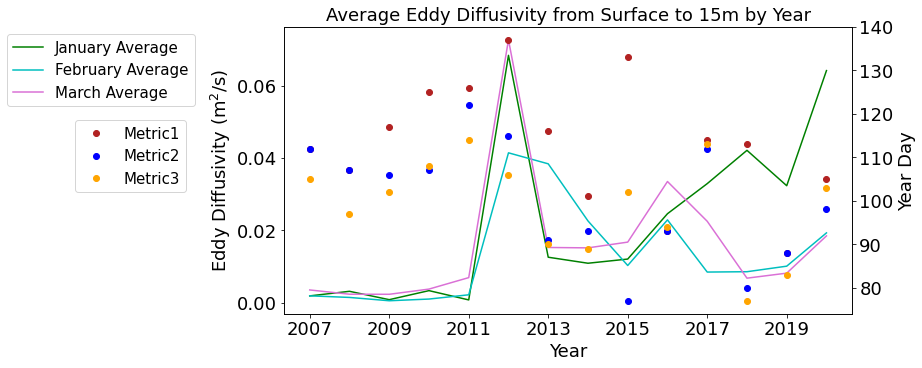
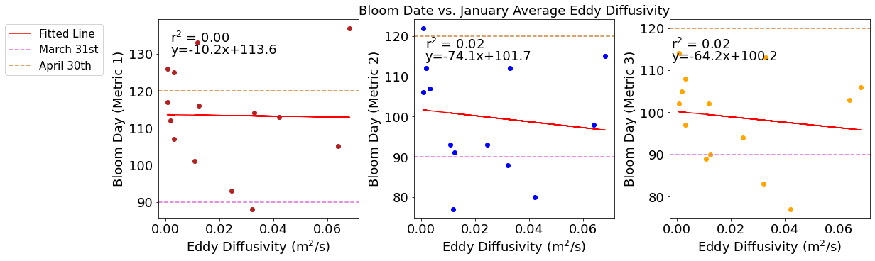
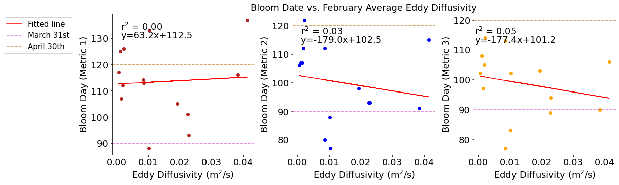
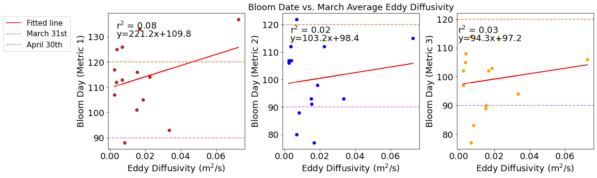
Monthly average eddy diffusivity in top 30m (January-March)
[28]:
fig,ax=plt.subplots(1,1,figsize=(12,5),constrained_layout=True)
p1=ax.plot(years,eddy30jan, '-',color='green',label='January Average')
p2=ax.plot(years,eddy30feb, '-',color='c',label='February Average')
p3=ax.plot(years,eddy30mar, '-',color='orchid',label='March Average')
ax.set_ylabel('Eddy Diffusivity ($\mathregular{m^2}$/s)')
ax.set_xlabel('Year')
ax.set_title('Average Eddy Diffusivity from Surface to 30m by Year')
ax.set_xticks([2007,2009,2011,2013,2015,2017,2019])
ax.legend(handles=[p1[0],p2[0],p3[0]],bbox_to_anchor=(-0.54, 1.0), loc='upper left')

ax1=ax.twinx()
p4=ax1.plot(years,yearday1, 'o',color='firebrick',label='Metric1')
p5=ax1.plot(years,yearday2, 'o',color='b',label='Metric2')
p6=ax1.plot(years,yearday3, 'o',color='orange',label='Metric3')
ax1.set_ylabel('Year Day')
ax1.legend(handles=[p4[0],p5[0],p6[0]],bbox_to_anchor=(-0.4, 0.7), loc='upper left')

# ---------- Jan ---------
fig2,ax2=plt.subplots(1,3,figsize=(17,5),constrained_layout=True)
ax2[0].plot(eddy30jan,yearday1,'o',color='firebrick')
ax2[0].set_xlabel('Eddy Diffusivity ($\mathregular{m^2}$/s)')
ax2[0].set_ylabel('Bloom Day (Metric 1)')
y,r2,m,b=bloomdrivers.reg_r2(eddy30jan,yearday1)
ax2[0].plot(eddy30jan, y, 'r', label='Fitted Line')
ax2[0].text(0.02, 0.9, '$\mathregular{r^2}$ = %.2f'%r2, transform=ax.transAxes)
ax2[0].text(0.02,0.83,f'y={round(m,1)}x+{round(b,1)}',horizontalalignment='left',verticalalignment='bottom',transform=ax.transAxes)

ax2[1].plot(eddy30jan,yearday2,'o',color='b')
ax2[1].set_xlabel('Eddy Diffusivity ($\mathregular{m^2}$/s)')
ax2[1].set_ylabel('Bloom Day (Metric 2)')
y,r2,m,b=bloomdrivers.reg_r2(eddy30jan,yearday2)
ax2[1].plot(eddy30jan, y, 'r', label='Fitted line')
ax2[1].text(0.65, 0.87, '$\mathregular{r^2}$ = %.2f'%r2, transform=ax.transAxes)
ax2[1].text(0.65,0.8,f'y={round(m,1)}x+{round(b,1)}',horizontalalignment='left',verticalalignment='bottom',transform=ax.transAxes)

ax2[2].plot(eddy30jan,yearday3,'o',color='orange')
ax2[2].set_xlabel('Eddy Diffusivity ($\mathregular{m^2}$/s)')
ax2[2].set_ylabel('Bloom Day (Metric 3)')
y,r2,m,b=bloomdrivers.reg_r2(eddy30jan,yearday3)
ax2[2].plot(eddy30jan, y, 'r', label='Fitted line')
ax2[2].text(1.26, 0.87, '$\mathregular{r^2}$ = %.2f'%r2, transform=ax.transAxes)
ax2[2].text(1.26,0.8,f'y={round(m,1)}x+{round(b,1)}',horizontalalignment='left',verticalalignment='bottom',transform=ax.transAxes)

ax2[1].set_title('Bloom Date vs. January Average Eddy Diffusivity')

# ---------- Feb ---------
fig3,ax3=plt.subplots(1,3,figsize=(17,5),constrained_layout=True)
ax3[0].plot(eddy30feb,yearday1,'o',color='firebrick')
ax3[0].set_xlabel('Eddy Diffusivity ($\mathregular{m^2}$/s)')
ax3[0].set_ylabel('Bloom Day (Metric 1)')
y,r2,m,b=bloomdrivers.reg_r2(eddy30feb,yearday1)
ax3[0].plot(eddy30feb, y, 'r', label='Fitted line')
ax3[0].text(0.02, 0.9, '$\mathregular{r^2}$ = %.2f'%r2, transform=ax.transAxes)
ax3[0].text(0.02,0.83,f'y={round(m,1)}x+{round(b,1)}',horizontalalignment='left',verticalalignment='bottom',transform=ax.transAxes)

ax3[1].plot(eddy30feb,yearday2,'o',color='b')
ax3[1].set_xlabel('Eddy Diffusivity ($\mathregular{m^2}$/s)')
ax3[1].set_ylabel('Bloom Day (Metric 2)')
y,r2,m,b=bloomdrivers.reg_r2(eddy30feb,yearday2)
ax3[1].plot(eddy30feb, y, 'r', label='Fitted line')
ax3[1].text(0.65, 0.87, '$\mathregular{r^2}$ = %.2f'%r2, transform=ax.transAxes)
ax3[1].text(0.65,0.8,f'y={round(m,1)}x+{round(b,1)}',horizontalalignment='left',verticalalignment='bottom',transform=ax.transAxes)

ax3[2].plot(eddy30feb,yearday3,'o',color='orange')
ax3[2].set_xlabel('Eddy Diffusivity ($\mathregular{m^2}$/s)')
ax3[2].set_ylabel('Bloom Day (Metric 3)')
y,r2,m,b=bloomdrivers.reg_r2(eddy30feb,yearday3)
ax3[2].plot(eddy30feb, y, 'r', label='Fitted line')
ax3[2].text(1.26, 0.87, '$\mathregular{r^2}$ = %.2f'%r2, transform=ax.transAxes)
ax3[2].text(1.26,0.8,f'y={round(m,1)}x+{round(b,1)}',horizontalalignment='left',verticalalignment='bottom',transform=ax.transAxes)

ax3[1].set_title('Bloom Date vs. February Average Eddy Diffusivity')

# ---------- March ---------
fig4,ax4=plt.subplots(1,3,figsize=(17,5),constrained_layout=True)
ax4[0].plot(eddy30mar,yearday1,'o',color='firebrick')
ax4[0].set_xlabel('Eddy Diffusivity ($\mathregular{m^2}$/s)')
ax4[0].set_ylabel('Bloom Day (Metric 1)')
y,r2,m,b=bloomdrivers.reg_r2(eddy30mar,yearday1)
ax4[0].plot(eddy30mar, y, 'r', label='Fitted line')
ax4[0].text(0.02, 0.9, '$\mathregular{r^2}$ = %.2f'%r2, transform=ax.transAxes)
ax4[0].text(0.02,0.83,f'y={round(m,1)}x+{round(b,1)}',horizontalalignment='left',verticalalignment='bottom',transform=ax.transAxes)

ax4[1].plot(eddy30mar,yearday2,'o',color='b')
ax4[1].set_xlabel('Eddy Diffusivity ($\mathregular{m^2}$/s)')
ax4[1].set_ylabel('Bloom Day (Metric 2)')
y,r2,m,b=bloomdrivers.reg_r2(eddy30mar,yearday2)
ax4[1].plot(eddy30mar, y, 'r', label='Fitted line')
ax4[1].text(0.65, 0.87, '$\mathregular{r^2}$ = %.2f'%r2, transform=ax.transAxes)
ax4[1].text(0.65,0.8,f'y={round(m,1)}x+{round(b,1)}',horizontalalignment='left',verticalalignment='bottom',transform=ax.transAxes)

ax4[2].plot(eddy30mar,yearday3,'o',color='orange')
ax4[2].set_xlabel('Eddy Diffusivity ($\mathregular{m^2}$/s)')
ax4[2].set_ylabel('Bloom Day (Metric 3)')
y,r2,m,b=bloomdrivers.reg_r2(eddy30mar,yearday3)
ax4[2].plot(eddy30mar, y, 'r', label='Fitted line')
ax4[2].text(1.26, 0.87, '$\mathregular{r^2}$ = %.2f'%r2, transform=ax.transAxes)
ax4[2].text(1.26,0.8,f'y={round(m,1)}x+{round(b,1)}',horizontalalignment='left',verticalalignment='bottom',transform=ax.transAxes)

ax4[1].set_title('Bloom Date vs. March Average Eddy Diffusivity')

# Jan month lines
ax2[0].axhline(y=90, color='orchid', linestyle='--',label='March 31st')
ax2[0].axhline(y=120, color='peru', linestyle='--',label='April 30th')
ax2[0].legend(bbox_to_anchor=(-0.25, 1.0))
ax2[1].axhline(y=90, color='orchid', linestyle='--')
ax2[2].axhline(y=90, color='orchid', linestyle='--',label='March 31st')
ax2[1].axhline(y=120, color='peru', linestyle='--')
ax2[2].axhline(y=120, color='peru', linestyle='--',label='April 30th')
# Feb month lines
ax3[0].axhline(y=90, color='orchid', linestyle='--',label='March 31st')
ax3[0].axhline(y=120, color='peru', linestyle='--',label='April 30th')
ax3[0].legend(bbox_to_anchor=(-0.25, 1.0))
ax3[1].axhline(y=90, color='orchid', linestyle='--')
ax3[2].axhline(y=90, color='orchid', linestyle='--',label='March 31st')
ax3[1].axhline(y=120, color='peru', linestyle='--')
ax3[2].axhline(y=120, color='peru', linestyle='--',label='April 30th')
# March month lines
ax4[0].axhline(y=90, color='orchid', linestyle='--',label='March 31st')
ax4[0].axhline(y=120, color='peru', linestyle='--',label='April 30th')
ax4[0].legend(bbox_to_anchor=(-0.25, 1.0))
ax4[1].axhline(y=90, color='orchid', linestyle='--')
ax4[2].axhline(y=90, color='orchid', linestyle='--',label='March 31st')
ax4[1].axhline(y=120, color='peru', linestyle='--')
ax4[2].axhline(y=120, color='peru', linestyle='--',label='April 30th')
[28]:
<matplotlib.lines.Line2D at 0x7f70f92cc910>
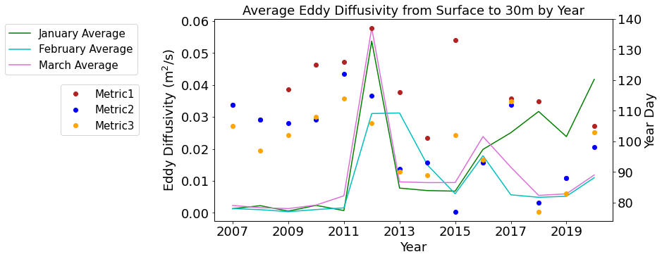


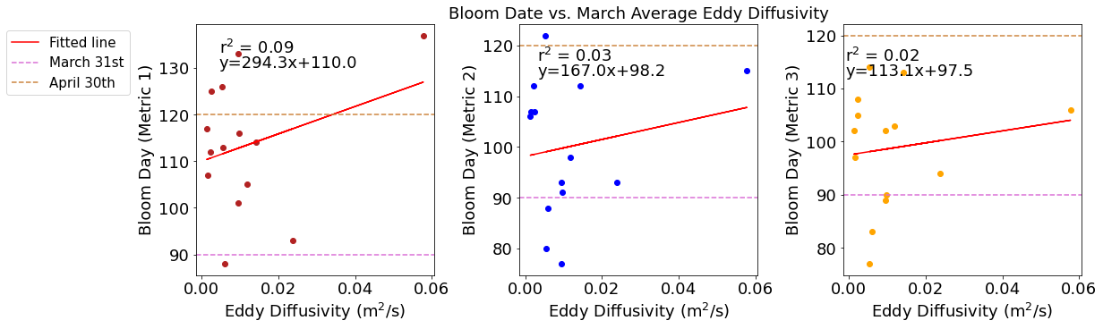
[ ]: