Central SoG Bloom Timing Analysis (Station S3)
Station S3 is a location off the central/south east coast of Vancouver Island. It was chosen as the first location to examine in order to compare to the results of a previous environmental driver analysis of spring bloom timing based on a 1-dimensional model [1] that served as a starting point from which the present 3-dimensional implementation was developed.
A time series of phytoplankton concentrations, environmental forcings and bloom timing at Station S3 from 2007-2020 can be found in this notebook. The environmental drivers were averaged over each month for January, February and March. It was found that the most significant relationships between bloom date and drivers occurred in March. This is apparent for solar radiation (Figure 1), as well as other bloom date versus environmental driver plots found in this time series notebook. Although a strong negative relationship between March zooplankton concentrations and bloom timing was observed, it was decided to not explore that correlation further, as the variation in zooplankton concentration was likely a direct result of the timing of the spring phytoplankton bloom.
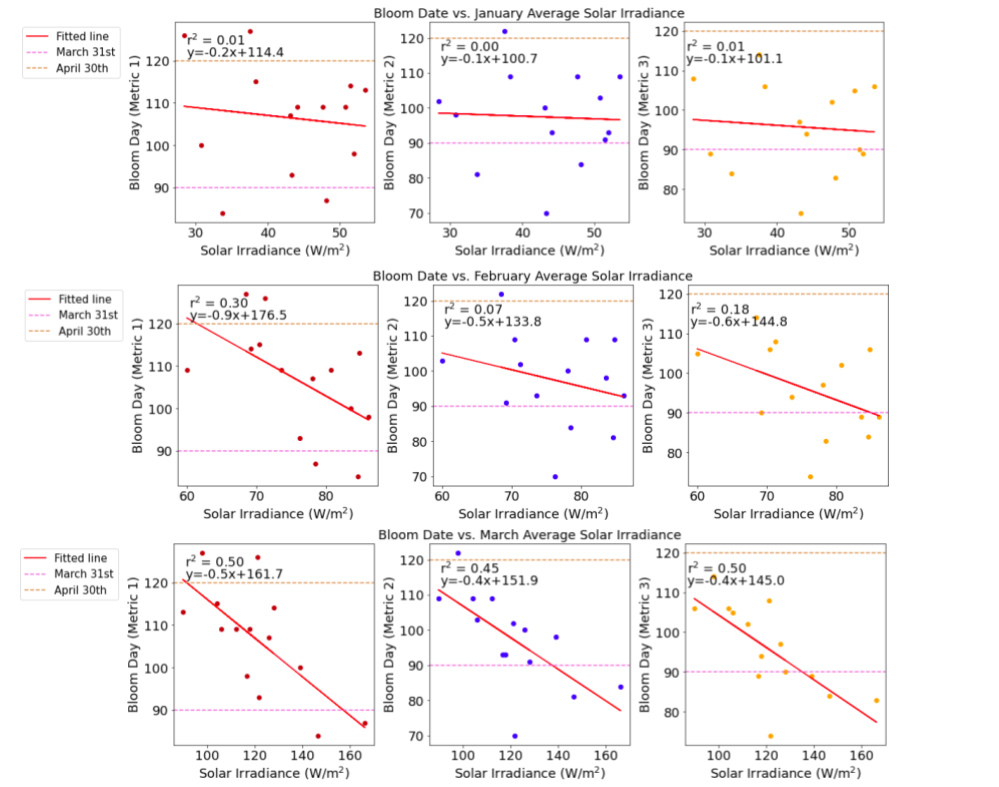
Figure 1. Correlation between monthly averaged solar radiation and bloom timing according to three different metrics. The bottom three plots show that the highest R-squared values of the regression between bloom date and average solar radiation occurs in March, relative to the regressions for January and February.
Next, correlation, residuals analysis and multiple linear regression (Table 1) were done on environmental forcings and bloom timing. The notebook can be found here. By looking at 3 correlation plots between bloom date and environmental driver averages for January, February and March, the most significant correlations were once again seen in the March averages (Figure 2).
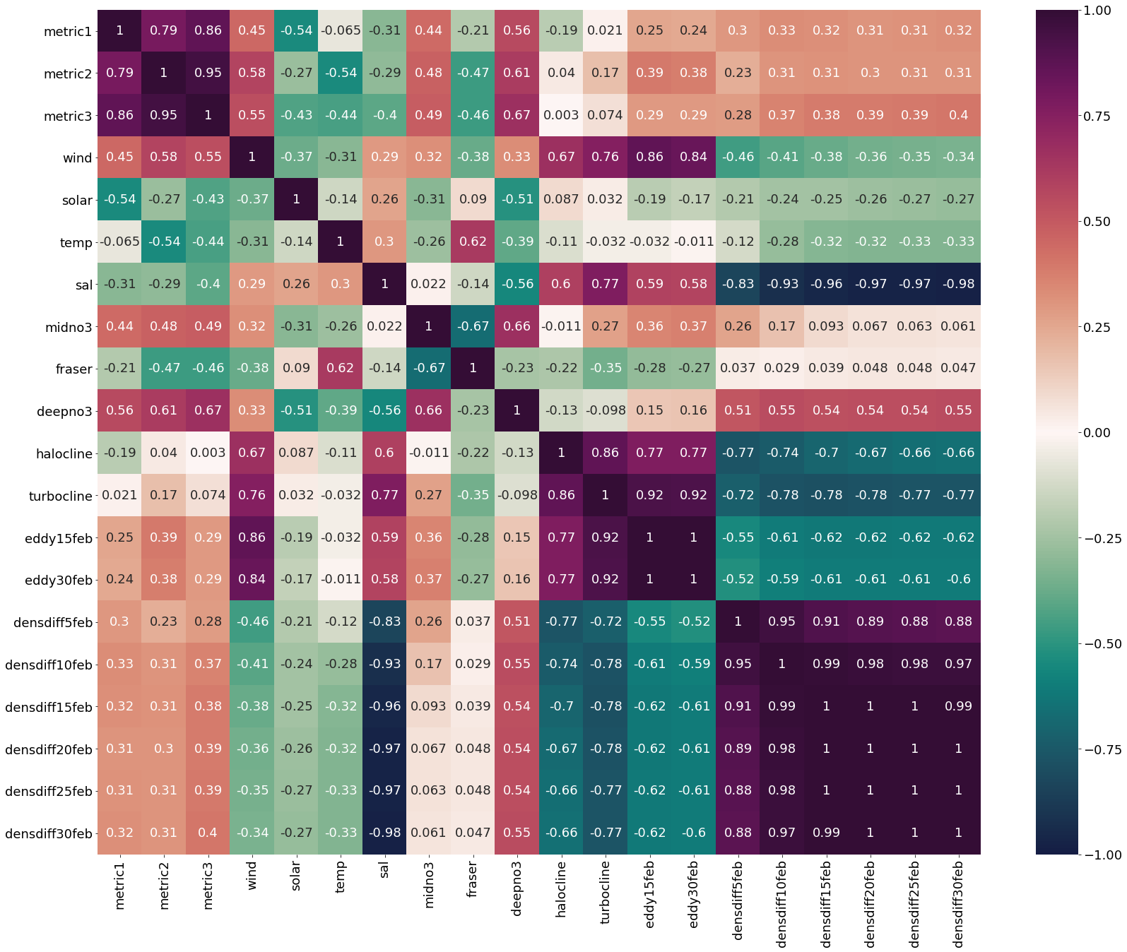
Figure 2. Heatmap of correlation coefficients between bloom dates for each definition (metric 1, metric 2 and metric 3) and environmental drivers averaged through March.
It was found that the most correlated driver with bloom date was wind speed cubed, with turbocline depth being a close second. While turbocline depth has strong correlations with bloom timing, it is also very highly correlated with wind speed variability. Due to the causal relationship between wind speeds and turbocline depth through wind driven mixing, our interpretation is that wind is the key environmental driver in this location. There is a strong positive relationship between wind and bloom timing because stronger wind leads to increased mixing near the surface (Figure 4). When phytoplankton are mixed to greater depth, their average exposure to light is reduced, leading to slower growth and a delayed bloom. Additionally, the surface phytoplankton concentration is reduced through dilution. In contrast, early stratification allows phytoplankton to remain concentrated near the surface and be exposed to greater light levels than when mixed to greater depths, leading to an earlier bloom.
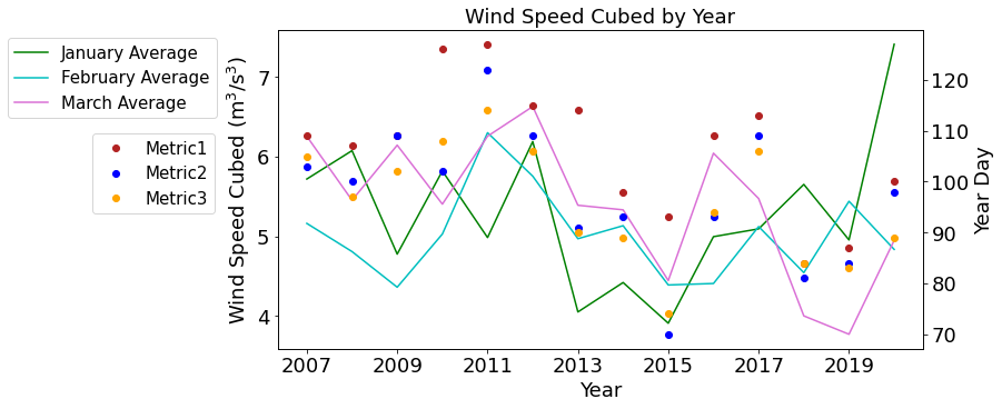
Figure 3. Time series from 2007-2020 of monthly averaged wind speed cubed (left axis) and bloom dates (right axis) according to three different metrics. The lines connecting the interannual variability in wind speed cubed hold no meaning, and are simply present to easily distinguish between the environmental driver and the bloom date.
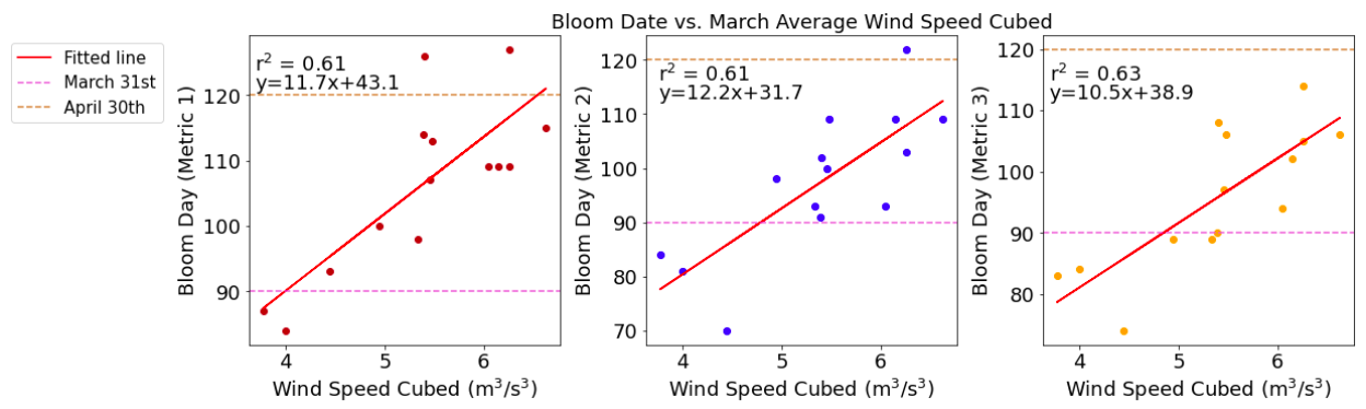
Figure 4. Correlation between March average wind speed cubed and spring phytoplankton bloom timing according to three different metrics. A positive relationship is observed between this environmental driver and bloom timing.
The next strongest correlation with bloom timing was solar radiation. Higher solar radiation (reduced cloud cover) in March exposes phytoplankton to greater light levels, which promotes faster growth and, consequently, an earlier bloom (Figure 1). Additionally, solar radiation increases near-surface temperature. Solar radiation is strongly anti-correlated with wind, meaning years with low winds also experience high solar radiation. These combining effects have a strong influence on bloom development.
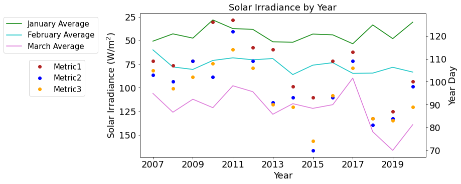
Figure 5. Time series from 2007-2020 of monthly averaged solar radiation (left axis) and bloom dates (right axis) according to three different metrics. The lines connecting the interannual variability in solar radiation hold no meaning, and are simply present to easily distinguish between the environmental driver and the bloom date.
Temperature itself was the third environmental condition that was highly correlated with bloom timing at station S3. Temperature is influenced by, and therefore correlated with, the previously discussed factors of wind speed and solar radiation. Additionally, surface temperature itself can influence bloom timing in multiple ways. All biological rates in the model have temperature dependence. Phytoplankton growth rates increase at warmer temperatures, but so do grazing and mortality. However, during the spring bloom period, a time of net primary production, the increase in phytoplankton growth rate at warmer temperatures can be expected to outweigh the increase in loss terms. Lower dominant zooplankton biomass has been observed during warmer years, which would decrease grazing pressure on phytoplankton and result in an earlier bloom [2]. Although temperature can affect stratification due to vertical differences in density, the effects are small compared to the temperature dependence on the rates of mortality, grazing and growth [1].
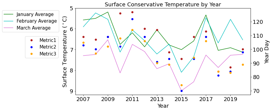
Figure 6. Time series from 2007-2020 of monthly averaged surface conservative temperature (left axis) and bloom dates (right axis) according to three different metrics. The lines connecting the interannual variability in surface temperature hold no meaning, and are simply present to easily distinguish between the environmental driver and the bloom date.
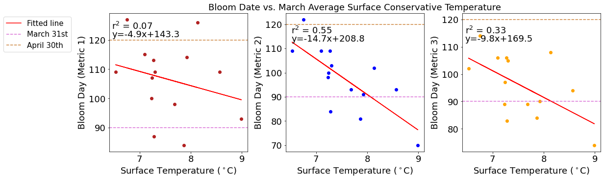
Figure 7. Correlation between March average surface conservative temperature and spring phytoplankton bloom timing according to three different metrics. A negative relationship is observed between this environmental driver and bloom timing.
Another possible tertiary environmental driver for spring bloom timing at station S3 is the Fraser river input. Although the Fraser flow initially had a weak correlation with bloom timing, residual analysis showed that when wind or solar radiation effects were subtracted, there was a strong negative relationship of the residuals with Fraser flow (Figure 8). The Fraser river is the most significant single source of freshwater to the Salish Sea. When Fraser flow rates are high in March, it creates strong stratification between low salinity surface waters and high salinity deep waters. Similarly to the effects of wind, this stratification allows phytoplankton to be mixed at shallower depths, which exposes them to more light and results in fast growth and an early bloom. Although mid-depth nitrate concentrations (30-90m) had high correlations with bloom timing, it was determined from examining a time series that the variation of this environmental factor likely resulted from rather than drove bloom timing.
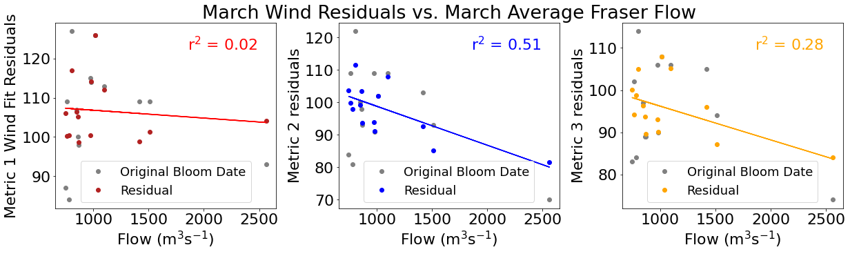
Figure 8. Correlation between March average Fraser river flow and spring phytoplankton bloom timing according to three different metrics (grey dots). Correlation between March average Fraser river flow and the residuals from regression of March wind speed cubed and bloom timing according to three different metrics (coloured dots). A negative relationship is observed between this environmental driver and bloom timing. This signifies that when the variability from wind is subtracted, a strong relationship between Fraser flow and bloom timing is observed.
In summary, this analysis identifies the four strongest environmental drivers of spring phytoplankton bloom timing at Station S3. The primary driver was found to be wind speeds, the secondary driver was solar radiation, and sea surface temperatures and Fraser flow rates were found to be equally strong tertiary drivers. This is partially consistent with the findings of Collins et. al (2009), which determined through analysis of a 1-D model at Station S3 that the primary driver of the spring bloom was wind speed, with solar radiation being a secondary driver [1]. They did not, however, find any effect from surface temperatures or Fraser input on phytoplankton bloom timing, whereas the present analysis did identify a strong impact from both of these factors. The effect of the Fraser River was parameterized in Collins et al. (2009) but is more fully represented in the present model, which could be a leading cause in this discrepancy.
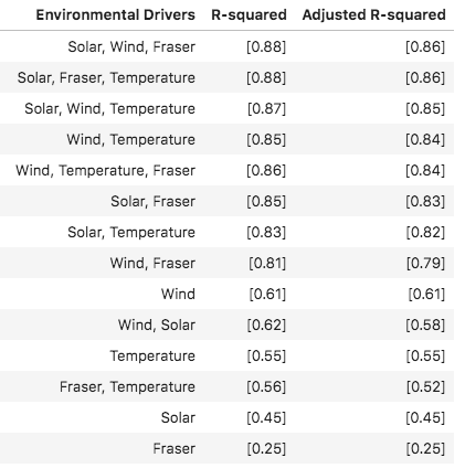
Table 1. R-squared and adjusted R-squared values from regression between bloom timing and one or more environmental drivers.
References: