Station QU39 analysis
An analysis of the environmental drivers of spring bloom timing at Station QU39. This notebook works only for variables stored in pickle files created by the notebook makePickles201905.ipynb, which can be found at /ocean/aisabell/MEOPAR/Analysis-Aline/notebooks/notebooks/Bloom_Timing/stationQU39/makePickles201905_QU39.ipynb
To recreate this notebook, first create the pickle files, then follow the instructions in the second code cell.
[1]:
import numpy as np
import matplotlib.pyplot as plt
import matplotlib.dates as mdates
import matplotlib as mpl
import netCDF4 as nc
import datetime as dt
from salishsea_tools import evaltools as et, places, viz_tools, visualisations, bloomdrivers
import xarray as xr
import pandas as pd
import pickle
import os
import seaborn as sns
import cmocean
import pylab


%matplotlib inline
To recreate this notebook at a different location
follow these instructions:
[2]:
# The path to the directory where the pickle files are stored:
savedir='/ocean/aisabell/MEOPAR/extracted_files'
# Change 'S3' to the location of interest
loc='QU39'
# What is the start year and end year+1 of the time range of interest?
startyear=2007
endyear=2021 # does NOT include this value

# Note: x and y limits on the location map may need to be changed
# Note: xticks in the plots will need to be changed
# Note: 201812 bloom timing variable load and plotting will also need to be removed
[3]:
modver='201905'
# lat and lon information for place:
lon,lat=places.PLACES[loc]['lon lat']
# get place information on SalishSeaCast grid:
ij,ii=places.PLACES[loc]['NEMO grid ji']
jw,iw=places.PLACES[loc]['GEM2.5 grid ji']
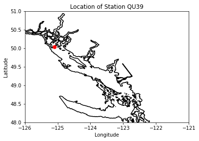
fig, ax = plt.subplots(1,1,figsize = (6,6))
with xr.open_dataset('/data/vdo/MEOPAR/NEMO-forcing/grid/mesh_mask201702.nc') as mesh:
ax.contour(mesh.nav_lon,mesh.nav_lat,mesh.tmask.isel(t=0,z=0),[0.1,],colors='k')
tmask=np.array(mesh.tmask)
gdept_1d=np.array(mesh.gdept_1d)
e3t_0=np.array(mesh.e3t_0)
ax.plot(lon, lat, '.', markersize=14, color='red')
ax.set_ylim(48,51)
ax.set_xlim(-126,-121)
ax.set_title('Location of Station %s'%loc)
ax.set_xlabel('Longitude')
ax.set_ylabel('Latitude')
viz_tools.set_aspect(ax,coords='map')
[3]:
1.1363636363636362
Strait of Georgia Region
[4]:
# define sog region:
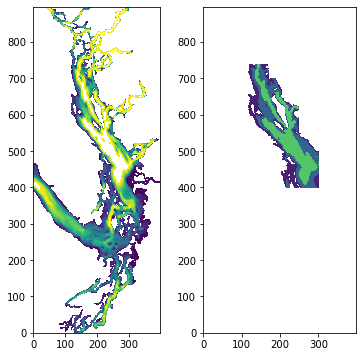
fig, ax = plt.subplots(1,2,figsize = (6,6))
with xr.open_dataset('/data/vdo/MEOPAR/NEMO-forcing/grid/bathymetry_201702.nc') as bathy:
bath=np.array(bathy.Bathymetry)
ax[0].contourf(bath,np.arange(0,250,10))
viz_tools.set_aspect(ax[0],coords='grid')
sogmask=np.copy(tmask[:,:,:,:])
sogmask[:,:,740:,:]=0
sogmask[:,:,700:,170:]=0
sogmask[:,:,550:,250:]=0
sogmask[:,:,:,302:]=0
sogmask[:,:,:400,:]=0
sogmask[:,:,:,:100]=0
#sogmask250[bath<250]=0
ax[1].contourf(np.ma.masked_where(sogmask[0,0,:,:]==0,bathy.Bathymetry),[0,100,250,550])
[4]:
<matplotlib.contour.QuadContourSet at 0x7f0219492a60>
[5]:
SMALL_SIZE = 15
MEDIUM_SIZE = 18
BIGGER_SIZE = 21

plt.rc('font', size=MEDIUM_SIZE)          # controls default text sizes
plt.rc('axes', titlesize=MEDIUM_SIZE)     # fontsize of the axes title
plt.rc('axes', labelsize=MEDIUM_SIZE)    # fontsize of the x and y labels
plt.rc('xtick', labelsize=MEDIUM_SIZE)    # fontsize of the tick labels
plt.rc('ytick', labelsize=MEDIUM_SIZE)    # fontsize of the tick labels
plt.rc('legend', fontsize=SMALL_SIZE)    # legend fontsize
plt.rc('figure', titlesize=BIGGER_SIZE)  # fontsize of the figure title
** Stop and check, have you made pickle files for all the years? **
[6]:
# loop through years of spring time series (mid feb-june) for bloom timing for 201905 run
years=list()
bloomtime1=list()
bloomtime2=list()
bloomtime3=list()
for year in range(startyear,endyear):
    fname3=f'springBloomTime_{str(year)}_{loc}_{modver}.pkl'
    savepath3=os.path.join(savedir,fname3)
    bio_time0,sno30,sdiat0,sflag0,scili0,diat_alld0,no3_alld0,flag_alld0,cili_alld0,phyto_alld0,\
                 intdiat0,intphyto0,fracdiat0,sphyto0,percdiat0=pickle.load(open(savepath3,'rb'))
    # put code that calculates bloom timing here
    bt1=bloomdrivers.metric1_bloomtime(phyto_alld0,no3_alld0,bio_time0)
    bt2=bloomdrivers.metric2_bloomtime(phyto_alld0,no3_alld0,bio_time0)
    bt3=bloomdrivers.metric3_bloomtime(sphyto0,sno30,bio_time0)
    years.append(year)
    bloomtime1.append(bt1)
    bloomtime2.append(bt2)
    bloomtime3.append(bt3)
years=np.array(years)
bloomtime1=np.array(bloomtime1)
bloomtime2=np.array(bloomtime2)
bloomtime3=np.array(bloomtime3)

# get year day
yearday1=et.datetimeToYD(bloomtime1)  # convert to year day tool
yearday2=et.datetimeToYD(bloomtime2)
yearday3=et.datetimeToYD(bloomtime3)
Combine separate year files into arrays:
[7]:
# loop through years (for location specific drivers)

years=list()
windjan=list()
windfeb=list()
windmar=list()
solarjan=list()
solarfeb=list()
solarmar=list()
parjan=list()
parfeb=list()
parmar=list()
tempjan=list()
tempfeb=list()
tempmar=list()
saljan=list()
salfeb=list()
salmar=list()
zoojan=list()
zoofeb=list()
zoomar=list()
mesozoojan=list()
mesozoofeb=list()
mesozoomar=list()
microzoojan=list()
microzoofeb=list()
microzoomar=list()
intzoojan=list()
intzoofeb=list()
intzoomar=list()
intmesozoojan=list()
intmesozoofeb=list()
intmesozoomar=list()
intmicrozoojan=list()
intmicrozoofeb=list()
intmicrozoomar=list()
midno3jan=list()
midno3feb=list()
midno3mar=list()

for year in range(startyear,endyear):
    fname=f'JanToMarch_TimeSeries_{year}_{loc}_{modver}.pkl'
    savepath=os.path.join(savedir,fname)
    bio_time,diat_alld,no3_alld,flag_alld,cili_alld,microzoo_alld,mesozoo_alld,\
            intdiat,intphyto,spar,intmesoz,intmicroz,grid_time,temp,salinity,u_wind,v_wind,twind,\
            solar,no3_30to90m,sno3,sdiat,sflag,scili,intzoop,fracdiat,zoop_alld,sphyto,phyto_alld,\
            percdiat,wspeed,winddirec=pickle.load(open(savepath,'rb'))
    # put code that calculates drivers here
    wind=bloomdrivers.D1_3monthly_avg(twind,wspeed)
    solar=bloomdrivers.D1_3monthly_avg(twind,solar)
    par=bloomdrivers.D1_3monthly_avg(bio_time,spar)
    temp=bloomdrivers.D1_3monthly_avg(grid_time,temp)
    sal=bloomdrivers.D1_3monthly_avg(grid_time,salinity)
    zoo=bloomdrivers.D2_3monthly_avg(bio_time,zoop_alld)
    mesozoo=bloomdrivers.D2_3monthly_avg(bio_time,mesozoo_alld)
    microzoo=bloomdrivers.D2_3monthly_avg(bio_time,microzoo_alld)
    intzoo=bloomdrivers.D1_3monthly_avg(bio_time,intzoop)
    intmesozoo=bloomdrivers.D1_3monthly_avg(bio_time,intmesoz)
    intmicrozoo=bloomdrivers.D1_3monthly_avg(bio_time,intmicroz)
    midno3=bloomdrivers.D1_3monthly_avg(bio_time,no3_30to90m)

    years.append(year)
    windjan.append(wind[0])
    windfeb.append(wind[1])
    windmar.append(wind[2])
    solarjan.append(solar[0])
    solarfeb.append(solar[1])
    solarmar.append(solar[2])
    parjan.append(par[0])
    parfeb.append(par[1])
    parmar.append(par[2])
    tempjan.append(temp[0])
    tempfeb.append(temp[1])
    tempmar.append(temp[2])
    saljan.append(sal[0])
    salfeb.append(sal[1])
    salmar.append(sal[2])
    zoojan.append(zoo[0])
    zoofeb.append(zoo[1])
    zoomar.append(zoo[2])
    mesozoojan.append(mesozoo[0])
    mesozoofeb.append(mesozoo[1])
    mesozoomar.append(mesozoo[2])
    microzoojan.append(microzoo[0])
    microzoofeb.append(microzoo[1])
    microzoomar.append(microzoo[2])
    intzoojan.append(intzoo[0])
    intzoofeb.append(intzoo[1])
    intzoomar.append(intzoo[2])
    intmesozoojan.append(intmesozoo[0])
    intmesozoofeb.append(intmesozoo[1])
    intmesozoomar.append(intmesozoo[2])
    intmicrozoojan.append(intmicrozoo[0])
    intmicrozoofeb.append(intmicrozoo[1])
    intmicrozoomar.append(intmicrozoo[2])
    midno3jan.append(midno3[0])
    midno3feb.append(midno3[1])
    midno3mar.append(midno3[2])

years=np.array(years)
windjan=np.array(windjan)
windfeb=np.array(windfeb)
windmar=np.array(windmar)
solarjan=np.array(solarjan)
solarfeb=np.array(solarfeb)
solarmar=np.array(solarmar)
parjan=np.array(parjan)
parfeb=np.array(parfeb)
parmar=np.array(parmar)
tempjan=np.array(tempjan)
tempfeb=np.array(tempfeb)
tempmar=np.array(tempmar)
saljan=np.array(saljan)
salfeb=np.array(salfeb)
salmar=np.array(salmar)
zoojan=np.array(zoojan)
zoofeb=np.array(zoofeb)
zoomar=np.array(zoomar)
mesozoojan=np.array(mesozoojan)
mesozoofeb=np.array(mesozoofeb)
mesozoomar=np.array(mesozoomar)
microzoojan=np.array(microzoojan)
microzoofeb=np.array(microzoofeb)
microzoomar=np.array(microzoomar)
intzoojan=np.array(intzoojan)
intzoofeb=np.array(intzoofeb)
intzoomar=np.array(intzoomar)
intmesozoojan=np.array(intmesozoojan)
intmesozoofeb=np.array(intmesozoofeb)
intmesozoomar=np.array(intmesozoomar)
intmicrozoojan=np.array(intmicrozoojan)
intmicrozoofeb=np.array(intmicrozoofeb)
intmicrozoomar=np.array(intmicrozoomar)
midno3jan=np.array(midno3jan)
midno3feb=np.array(midno3feb)
midno3mar=np.array(midno3mar)
[8]:
# loop through years (for non-location specific drivers)
fraserjan=list()
fraserfeb=list()
frasermar=list()
deepno3jan=list()
deepno3feb=list()
deepno3mar=list()

for year in range(startyear,endyear):
    fname2=f'JanToMarch_TimeSeries_{year}_{modver}.pkl'
    savepath2=os.path.join(savedir,fname2)
    no3_past250m,riv_time,rivFlow=pickle.load(open(savepath2,'rb'))
    # Code that calculates drivers here
    fraser=bloomdrivers.D1_3monthly_avg2(riv_time,rivFlow)
    fraserjan.append(fraser[0])
    fraserfeb.append(fraser[1])
    frasermar.append(fraser[2])

    fname=f'JanToMarch_TimeSeries_{year}_{loc}_{modver}.pkl'
    savepath=os.path.join(savedir,fname)
    bio_time,diat_alld,no3_alld,flag_alld,cili_alld,microzoo_alld,mesozoo_alld,\
            intdiat,intphyto,spar,intmesoz,intmicroz,grid_time,temp,salinity,u_wind,v_wind,twind,\
            solar,no3_30to90m,sno3,sdiat,sflag,scili,intzoop,fracdiat,zoop_alld,sphyto,phyto_alld,\
            percdiat,wspeed,winddirec=pickle.load(open(savepath,'rb'))
    deepno3=bloomdrivers.D1_3monthly_avg(bio_time,no3_past250m)

    deepno3jan.append(deepno3[0])
    deepno3feb.append(deepno3[1])
    deepno3mar.append(deepno3[2])

fraserjan=np.array(fraserjan)
fraserfeb=np.array(fraserfeb)
frasermar=np.array(frasermar)
deepno3jan=np.array(deepno3jan)
deepno3feb=np.array(deepno3feb)
deepno3mar=np.array(deepno3mar)
Load mixing variables
[9]:
# for T grid depth:
startd=dt.datetime(2015,1,1) # some date to get depth
endd=dt.datetime(2015,1,2)
basedir='/results2/SalishSea/nowcast-green.201905/'
nam_fmt='nowcast'
flen=1 # files contain 1 day of data each
tres=24 # 1: hourly resolution; 24: daily resolution
flist=et.index_model_files(startd,endd,basedir,nam_fmt,flen,"grid_T",tres)
with xr.open_mfdataset(flist['paths']) as gridt:
    depth_T=np.array(gridt.deptht)

# loop through years (for mixing drivers)

halojan=list()
halofeb=list()
halomar=list()
turbojan=list()
turbofeb=list()
turbomar=list()
densdiff5jan=list()
densdiff10jan=list()
densdiff15jan=list()
densdiff20jan=list()
densdiff25jan=list()
densdiff30jan=list()
densdiff5feb=list()
densdiff10feb=list()
densdiff15feb=list()
densdiff20feb=list()
densdiff25feb=list()
densdiff30feb=list()
densdiff5mar=list()
densdiff10mar=list()
densdiff15mar=list()
densdiff20mar=list()
densdiff25mar=list()
densdiff30mar=list()
eddy15jan=list()
eddy15feb=list()
eddy15mar=list()
eddy30jan=list()
eddy30feb=list()
eddy30mar=list()

for year in range(startyear,endyear):
    fname4=f'JanToMarch_Mixing_{year}_{loc}_{modver}.pkl'
    savepath4=os.path.join(savedir,fname4)
    halocline,eddy,depth,grid_time,temp,salinity=pickle.load(open(savepath4,'rb'))

    # halocline
    halo=bloomdrivers.D1_3monthly_avg(grid_time,halocline)
    halojan.append(halo[0])
    halofeb.append(halo[1])
    halomar.append(halo[2])
    # turbocline
    turbo=bloomdrivers.turbo(eddy,grid_time,depth_T)
    turbojan.append(turbo[0])
    turbofeb.append(turbo[1])
    turbomar.append(turbo[2])
    # density differences
    dict_diffs=bloomdrivers.density_diff(salinity,temp,grid_time)
    values=dict_diffs.values()
    all_diffs=list(values)
    densdiff5jan.append(all_diffs[0])
    densdiff10jan.append(all_diffs[3])
    densdiff15jan.append(all_diffs[6])
    densdiff20jan.append(all_diffs[9])
    densdiff25jan.append(all_diffs[12])
    densdiff30jan.append(all_diffs[15])
    densdiff5feb.append(all_diffs[1])
    densdiff10feb.append(all_diffs[4])
    densdiff15feb.append(all_diffs[7])
    densdiff20feb.append(all_diffs[10])
    densdiff25feb.append(all_diffs[13])
    densdiff30feb.append(all_diffs[16])
    densdiff5mar.append(all_diffs[2])
    densdiff10mar.append(all_diffs[5])
    densdiff15mar.append(all_diffs[8])
    densdiff20mar.append(all_diffs[11])
    densdiff25mar.append(all_diffs[14])
    densdiff30mar.append(all_diffs[17])
    # average eddy diffusivity
    avg_eddy=bloomdrivers.avg_eddy(eddy,grid_time,ij,ii)
    eddy15jan.append(avg_eddy[0])
    eddy15feb.append(avg_eddy[1])
    eddy15mar.append(avg_eddy[2])
    eddy30jan.append(avg_eddy[3])
    eddy30feb.append(avg_eddy[4])
    eddy30mar.append(avg_eddy[5])

halojan=np.array(halojan)
halofeb=np.array(halofeb)
halomar=np.array(halomar)
turbojan=np.array(turbojan)
turbofeb=np.array(turbofeb)
turbomar=np.array(turbomar)
densdiff5jan=np.array(densdiff5jan)
densdiff10jan=np.array(densdiff10jan)
densdiff15jan=np.array(densdiff15jan)
densdiff20jan=np.array(densdiff20jan)
densdiff25jan=np.array(densdiff25jan)
densdiff30jan=np.array(densdiff30jan)
densdiff5feb=np.array(densdiff5feb)
densdiff10feb=np.array(densdiff10feb)
densdiff15feb=np.array(densdiff15feb)
densdiff20feb=np.array(densdiff20feb)
densdiff25feb=np.array(densdiff25feb)
densdiff30feb=np.array(densdiff30feb)
densdiff5mar=np.array(densdiff5mar)
densdiff10mar=np.array(densdiff10mar)
densdiff15mar=np.array(densdiff15mar)
densdiff20mar=np.array(densdiff20mar)
densdiff25mar=np.array(densdiff25mar)
densdiff30mar=np.array(densdiff30mar)
eddy15jan=np.array(eddy15jan)
eddy15feb=np.array(eddy15feb)
eddy15mar=np.array(eddy15mar)
eddy30jan=np.array(eddy30jan)
eddy30feb=np.array(eddy30feb)
eddy30mar=np.array(eddy30mar)
[10]:
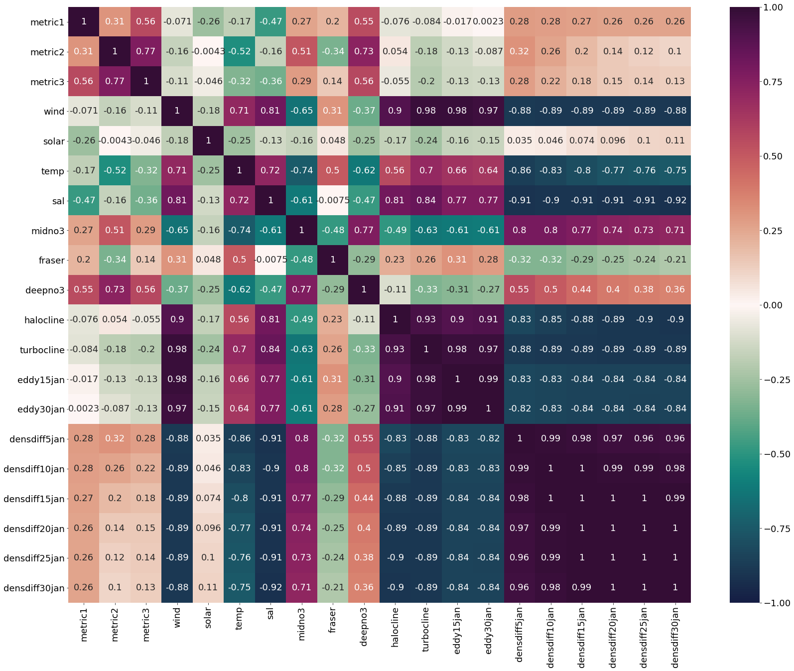
# January dataframe
dfjan=pd.DataFrame({'metric1':yearday1, 'metric2':yearday2, 'metric3':yearday3, 'wind':windjan,'solar':solarjan,
'temp':tempjan,'sal':saljan,'midno3':midno3jan,'fraser':fraserjan,'deepno3':deepno3jan,'halocline':halojan,
'turbocline':turbojan,'eddy15jan':eddy15jan,'eddy30jan':eddy30jan,'densdiff5jan':densdiff5jan,'densdiff10jan':densdiff10jan,
'densdiff15jan':densdiff15jan,'densdiff20jan':densdiff20jan,'densdiff25jan':densdiff25jan,'densdiff30jan':densdiff30jan})
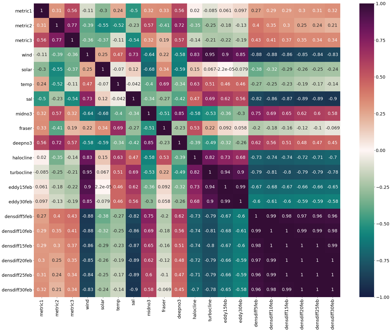
# February dataframe
dffeb=pd.DataFrame({'metric1':yearday1, 'metric2':yearday2, 'metric3':yearday3, 'wind':windfeb,'solar':solarfeb,
'temp':tempfeb,'sal':salfeb,'midno3':midno3feb,'fraser':fraserfeb,'deepno3':deepno3feb,'halocline':halofeb,
'turbocline':turbofeb,'eddy15feb':eddy15feb,'eddy30feb':eddy30feb,'densdiff5feb':densdiff5feb,'densdiff10feb':densdiff10feb,
'densdiff15feb':densdiff15feb,'densdiff20feb':densdiff20feb,'densdiff25feb':densdiff25feb,'densdiff30feb':densdiff30feb})
# March dataframe
dfmar=pd.DataFrame({'Metric1':yearday1, 'Metric2':yearday2, 'Metric3':yearday3, 'Wind':windmar,'Solar':solarmar,
'Temp':tempmar,'Salinity':salmar,'Mid NO3':midno3mar,'Fraser':frasermar,'Deep NO3':deepno3mar,'Halocline':halomar,
'Turbocline':turbomar,'Eddy 15m':eddy15mar,'Eddy 30m':eddy30mar,'Dens diff 5m':densdiff5mar,'Dens diff 10m':densdiff10mar,
'Dens diff 15m':densdiff15mar,'Dens diff 20m':densdiff20mar,'Dens diff 25m':densdiff25mar,'Dens diff 30m':densdiff30mar})
[11]:
dfjan.cov()
[11]:
| metric1 | metric2 | metric3 | wind | solar | temp | sal | midno3 | fraser | deepno3 | halocline | turbocline | eddy15jan | eddy30jan | densdiff5jan | densdiff10jan | densdiff15jan | densdiff20jan | densdiff25jan | densdiff30jan | |
|---|---|---|---|---|---|---|---|---|---|---|---|---|---|---|---|---|---|---|---|---|
| metric1 | 198.708791 | 58.818681 | 86.543956 | -1.781007 | -24.551781 | -1.899305 | -4.171853 | 3.182167 | 460.748634 | 7.319341 | -14.028757 | -10.208520 | -0.005371 | 0.000546 | 1.489626 | 1.996308 | 2.079153 | 2.035085 | 2.015683 | 2.006130 |
| metric2 | 58.818681 | 183.609890 | 114.093407 | -3.759146 | -0.392339 | -5.556492 | -1.366552 | 5.909751 | -735.152037 | 9.249013 | 9.568067 | -21.019686 | -0.039168 | -0.020004 | 1.609624 | 1.804854 | 1.437595 | 1.063485 | 0.914941 | 0.760366 |
| metric3 | 86.543956 | 114.093407 | 120.796703 | -2.198781 | -3.433917 | -2.763616 | -2.456685 | 2.671314 | 251.183023 | 5.807583 | -7.939469 | -18.687149 | -0.033942 | -0.024496 | 1.129664 | 1.243871 | 1.056110 | 0.885142 | 0.829251 | 0.791165 |
| wind | -1.781007 | -3.759146 | -2.198781 | 3.134961 | -2.107447 | 0.981135 | 0.901448 | -0.974413 | 88.585947 | -0.612914 | 20.890352 | 14.974924 | 0.039996 | 0.029182 | -0.580268 | -0.796133 | -0.855116 | -0.865071 | -0.862337 | -0.850927 |
| solar | -24.551781 | -0.392339 | -3.433917 | -2.107447 | 45.519190 | -1.330414 | -0.558300 | -0.899332 | 51.996331 | -1.589763 | -14.993866 | -14.146827 | -0.024421 | -0.017253 | 0.088360 | 0.157401 | 0.272019 | 0.356692 | 0.385514 | 0.413930 |
| temp | -1.899305 | -5.556492 | -2.763616 | 0.981135 | -1.330414 | 0.610327 | 0.350412 | -0.490322 | 62.318564 | -0.453589 | 5.746611 | 4.698350 | 0.011770 | 0.008494 | -0.252032 | -0.329667 | -0.340281 | -0.331984 | -0.326174 | -0.317574 |
| sal | -4.171853 | -1.366552 | -2.456685 | 0.901448 | -0.558300 | 0.350412 | 0.391185 | -0.325314 | -0.749033 | -0.277982 | 6.609216 | 4.504982 | 0.011022 | 0.008235 | -0.211624 | -0.286016 | -0.308297 | -0.313362 | -0.313584 | -0.312134 |
| midno3 | 3.182167 | 5.909751 | 2.671314 | -0.974413 | -0.899332 | -0.490322 | -0.325314 | 0.722836 | -65.951011 | 0.616738 | -5.451585 | -4.602925 | -0.011950 | -0.008816 | 0.252452 | 0.343353 | 0.354370 | 0.345060 | 0.338895 | 0.330073 |
| fraser | 460.748634 | -735.152037 | 251.183023 | 88.585947 | 51.996331 | 62.318564 | -0.749033 | -65.951011 | 25704.091440 | -43.359271 | 479.546075 | 355.694741 | 1.153008 | 0.777520 | -19.199387 | -26.115336 | -24.970412 | -22.344248 | -20.872513 | -18.740164 |
| deepno3 | 7.319341 | 9.249013 | 5.807583 | -0.612914 | -1.589763 | -0.453589 | -0.277982 | 0.616738 | -43.359271 | 0.880773 | -1.311233 | -2.700664 | -0.006737 | -0.004386 | 0.193277 | 0.236574 | 0.225218 | 0.204758 | 0.195887 | 0.185586 |
| halocline | -14.028757 | 9.568067 | -7.939469 | 20.890352 | -14.993866 | 5.746611 | 6.609216 | -5.451585 | 479.546075 | -1.311233 | 171.110379 | 104.798093 | 0.270881 | 0.203500 | -4.026102 | -5.677145 | -6.229664 | -6.406050 | -6.427093 | -6.393390 |
| turbocline | -10.208520 | -21.019686 | -18.687149 | 14.974924 | -14.146827 | 4.698350 | 4.504982 | -4.602925 | 355.694741 | -2.700664 | 104.798093 | 73.886129 | 0.192921 | 0.142397 | -2.814911 | -3.867555 | -4.161289 | -4.220687 | -4.214060 | -4.170163 |
| eddy15jan | -0.005371 | -0.039168 | -0.033942 | 0.039996 | -0.024421 | 0.011770 | 0.011022 | -0.011950 | 1.153008 | -0.006737 | 0.270881 | 0.192921 | 0.000529 | 0.000390 | -0.007079 | -0.009749 | -0.010477 | -0.010613 | -0.010585 | -0.010451 |
| eddy30jan | 0.000546 | -0.020004 | -0.024496 | 0.029182 | -0.017253 | 0.008494 | 0.008235 | -0.008816 | 0.777520 | -0.004386 | 0.203500 | 0.142397 | 0.000390 | 0.000291 | -0.005244 | -0.007229 | -0.007786 | -0.007907 | -0.007899 | -0.007817 |
| densdiff5jan | 1.489626 | 1.609624 | 1.129664 | -0.580268 | 0.088360 | -0.252032 | -0.211624 | 0.252452 | -19.199387 | 0.193277 | -4.026102 | -2.814911 | -0.007079 | -0.005244 | 0.139131 | 0.187908 | 0.198885 | 0.198567 | 0.197075 | 0.194085 |
| densdiff10jan | 1.996308 | 1.804854 | 1.243871 | -0.796133 | 0.157401 | -0.329667 | -0.286016 | 0.343353 | -26.115336 | 0.236574 | -5.677145 | -3.867555 | -0.009749 | -0.007229 | 0.187908 | 0.257906 | 0.275253 | 0.276186 | 0.274532 | 0.270761 |
| densdiff15jan | 2.079153 | 1.437595 | 1.056110 | -0.855116 | 0.272019 | -0.340281 | -0.308297 | 0.354370 | -24.970412 | 0.225218 | -6.229664 | -4.161289 | -0.010477 | -0.007786 | 0.198885 | 0.275253 | 0.295902 | 0.298437 | 0.297209 | 0.293715 |
| densdiff20jan | 2.035085 | 1.063485 | 0.885142 | -0.865071 | 0.356692 | -0.331984 | -0.313362 | 0.345060 | -22.344248 | 0.204758 | -6.406050 | -4.220687 | -0.010613 | -0.007907 | 0.198567 | 0.276186 | 0.298437 | 0.302231 | 0.301466 | 0.298438 |
| densdiff25jan | 2.015683 | 0.914941 | 0.829251 | -0.862337 | 0.385514 | -0.326174 | -0.313584 | 0.338895 | -20.872513 | 0.195887 | -6.427093 | -4.214060 | -0.010585 | -0.007899 | 0.197075 | 0.274532 | 0.297209 | 0.301466 | 0.300897 | 0.298097 |
| densdiff30jan | 2.006130 | 0.760366 | 0.791165 | -0.850927 | 0.413930 | -0.317574 | -0.312134 | 0.330073 | -18.740164 | 0.185586 | -6.393390 | -4.170163 | -0.010451 | -0.007817 | 0.194085 | 0.270761 | 0.293715 | 0.298438 | 0.298097 | 0.295594 |
[12]:
dffeb.cov()
[12]:
| metric1 | metric2 | metric3 | wind | solar | temp | sal | midno3 | fraser | deepno3 | halocline | turbocline | eddy15feb | eddy30feb | densdiff5feb | densdiff10feb | densdiff15feb | densdiff20feb | densdiff25feb | densdiff30feb | |
|---|---|---|---|---|---|---|---|---|---|---|---|---|---|---|---|---|---|---|---|---|
| metric1 | 198.708791 | 58.818681 | 86.543956 | -1.849740 | -41.773812 | 2.342734 | -3.239866 | 3.572518 | 1649.803298 | 7.411141 | 1.585195 | -5.660840 | 0.011697 | 0.014511 | 1.246483 | 1.685212 | 1.658779 | 1.660655 | 1.679456 | 1.699027 |
| metric2 | 58.818681 | 183.609890 | 114.093407 | -6.291101 | -74.793705 | -4.900849 | -1.419273 | 6.055971 | -1962.276543 | 9.132885 | -26.980415 | -16.081202 | -0.033107 | -0.018400 | 1.777272 | 1.955536 | 1.644143 | 1.339660 | 1.222098 | 1.071362 |
| metric3 | 86.543956 | 114.093407 | 120.796703 | -4.642330 | -40.508822 | -0.828064 | -2.734266 | 2.779492 | 738.413509 | 5.820826 | -9.073753 | -11.118173 | -0.032819 | -0.021803 | 1.556998 | 1.838885 | 1.648449 | 1.489859 | 1.447763 | 1.403427 |
| wind | -1.849740 | -6.291101 | -4.642330 | 1.401925 | 2.911385 | 0.381466 | 0.398035 | -0.593709 | 89.382727 | -0.644834 | 5.615016 | 5.308898 | 0.014548 | 0.010689 | -0.343006 | -0.423413 | -0.410310 | -0.389914 | -0.381788 | -0.369598 |
| solar | -41.773812 | -74.793705 | -40.508822 | 2.911385 | 99.145234 | -0.482920 | 0.559377 | -5.327000 | 1168.686718 | -5.520401 | 8.598186 | 3.159787 | -0.000003 | -0.008327 | -1.232965 | -1.313714 | -1.139214 | -0.987906 | -0.939278 | -0.879533 |
| temp | 2.342734 | -4.900849 | -0.828064 | 0.381466 | -0.482920 | 0.478955 | -0.013275 | -0.215094 | 167.352499 | -0.220183 | 2.486131 | 1.668419 | 0.004312 | 0.003354 | -0.060687 | -0.071531 | -0.063301 | -0.050422 | -0.044022 | -0.035415 |
| sal | -3.239866 | -1.419273 | -2.734266 | 0.398035 | 0.559377 | -0.013275 | 0.212630 | -0.123869 | -42.880221 | -0.179813 | 1.243835 | 1.497781 | 0.003892 | 0.002761 | -0.124445 | -0.161186 | -0.161406 | -0.158466 | -0.157484 | -0.155511 |
| midno3 | 3.572518 | 6.055971 | 2.779492 | -0.593709 | -5.327000 | -0.215094 | -0.123869 | 0.617537 | -140.013352 | 0.622136 | -2.584556 | -1.957714 | -0.003794 | -0.002469 | 0.192130 | 0.221361 | 0.205215 | 0.187614 | 0.180807 | 0.171595 |
| fraser | 1649.803298 | -1962.276543 | 738.413509 | 89.382727 | 1168.686718 | 167.352499 | -42.880221 | -140.013352 | 122323.912955 | -76.481005 | 1063.033169 | 363.471527 | 0.436726 | 0.213553 | -23.407139 | -25.651198 | -22.482233 | -16.675317 | -13.482208 | -9.090725 |
| deepno3 | 7.411141 | 9.132885 | 5.820826 | -0.644834 | -5.520401 | -0.220183 | -0.179813 | 0.622136 | -76.481005 | 0.869508 | -2.063388 | -2.141814 | -0.004073 | -0.002606 | 0.189213 | 0.213784 | 0.192431 | 0.173443 | 0.166751 | 0.157513 |
| halocline | 1.585195 | -26.980415 | -9.073753 | 5.615016 | 8.598186 | 2.486131 | 1.243835 | -2.584556 | 1063.033169 | -2.063388 | 32.428055 | 21.959424 | 0.056677 | 0.041261 | -1.356287 | -1.716491 | -1.683829 | -1.600741 | -1.559671 | -1.496221 |
| turbocline | -5.660840 | -16.081202 | -11.118173 | 5.308898 | 3.159787 | 1.668419 | 1.497781 | -1.957714 | 363.471527 | -2.141814 | 21.959424 | 22.141375 | 0.060089 | 0.045044 | -1.226140 | -1.549798 | -1.518873 | -1.449962 | -1.419688 | -1.373728 |
| eddy15feb | 0.011697 | -0.033107 | -0.032819 | 0.014548 | -0.000003 | 0.004312 | 0.003892 | -0.003794 | 0.436726 | -0.004073 | 0.056677 | 0.060089 | 0.000185 | 0.000143 | -0.002978 | -0.003779 | -0.003683 | -0.003507 | -0.003433 | -0.003329 |
| eddy30feb | 0.014511 | -0.018400 | -0.021803 | 0.010689 | -0.008327 | 0.003354 | 0.002761 | -0.002469 | 0.213553 | -0.002606 | 0.041261 | 0.045044 | 0.000143 | 0.000112 | -0.002081 | -0.002649 | -0.002574 | -0.002444 | -0.002390 | -0.002317 |
| densdiff5feb | 1.246483 | 1.777272 | 1.556998 | -0.343006 | -1.232965 | -0.060687 | -0.124445 | 0.192130 | -23.407139 | 0.189213 | -1.356287 | -1.226140 | -0.002978 | -0.002081 | 0.107635 | 0.132475 | 0.129206 | 0.123422 | 0.121117 | 0.117651 |
| densdiff10feb | 1.685212 | 1.955536 | 1.838885 | -0.423413 | -1.313714 | -0.071531 | -0.161186 | 0.221361 | -25.651198 | 0.213784 | -1.716491 | -1.549798 | -0.003779 | -0.002649 | 0.132475 | 0.165475 | 0.162745 | 0.156326 | 0.153676 | 0.149582 |
| densdiff15feb | 1.658779 | 1.644143 | 1.648449 | -0.410310 | -1.139214 | -0.063301 | -0.161406 | 0.205215 | -22.482233 | 0.192431 | -1.683829 | -1.518873 | -0.003683 | -0.002574 | 0.129206 | 0.162745 | 0.161085 | 0.155455 | 0.153067 | 0.149260 |
| densdiff20feb | 1.660655 | 1.339660 | 1.489859 | -0.389914 | -0.987906 | -0.050422 | -0.158466 | 0.187614 | -16.675317 | 0.173443 | -1.600741 | -1.449962 | -0.003507 | -0.002444 | 0.123422 | 0.156326 | 0.155455 | 0.150692 | 0.148656 | 0.145294 |
| densdiff25feb | 1.679456 | 1.222098 | 1.447763 | -0.381788 | -0.939278 | -0.044022 | -0.157484 | 0.180807 | -13.482208 | 0.166751 | -1.559671 | -1.419688 | -0.003433 | -0.002390 | 0.121117 | 0.153676 | 0.153067 | 0.148656 | 0.146783 | 0.143634 |
| densdiff30feb | 1.699027 | 1.071362 | 1.403427 | -0.369598 | -0.879533 | -0.035415 | -0.155511 | 0.171595 | -9.090725 | 0.157513 | -1.496221 | -1.373728 | -0.003329 | -0.002317 | 0.117651 | 0.149582 | 0.149260 | 0.145294 | 0.143634 | 0.140786 |
[13]:
dfmar.cov()
[13]:
| Metric1 | Metric2 | Metric3 | Wind | Solar | Temp | Salinity | Mid NO3 | Fraser | Deep NO3 | Halocline | Turbocline | Eddy 15m | Eddy 30m | Dens diff 5m | Dens diff 10m | Dens diff 15m | Dens diff 20m | Dens diff 25m | Dens diff 30m | |
|---|---|---|---|---|---|---|---|---|---|---|---|---|---|---|---|---|---|---|---|---|
| Metric1 | 198.708791 | 58.818681 | 86.543956 | 4.365834 | -185.218296 | 0.013832 | -0.290914 | 2.136903 | 2017.992998 | 7.361070 | 71.198823 | 28.176383 | 0.076010 | 0.063054 | 0.171061 | -0.007819 | -0.353067 | -0.600573 | -0.687358 | -0.799498 |
| Metric2 | 58.818681 | 183.609890 | 114.093407 | 1.813381 | -230.751058 | -4.922801 | 1.633999 | 5.690149 | -2441.123281 | 9.106444 | 85.613449 | 15.828831 | 0.035473 | 0.035777 | -0.098475 | -0.826942 | -1.364141 | -1.778049 | -1.919407 | -2.071328 |
| Metric3 | 86.543956 | 114.093407 | 120.796703 | 3.582495 | -219.604300 | -1.512966 | 0.389586 | 1.891126 | 974.083020 | 5.845356 | 56.099428 | 20.100823 | 0.032414 | 0.024222 | -0.097452 | -0.640954 | -1.044427 | -1.350948 | -1.447003 | -1.550702 |
| Wind | 4.365834 | 1.813381 | 3.582495 | 1.909641 | -3.958546 | 0.146660 | -0.047482 | -0.399715 | 199.635382 | -0.193218 | 11.378855 | 7.881106 | 0.023026 | 0.017404 | -0.115616 | -0.169596 | -0.179415 | -0.176016 | -0.175132 | -0.172940 |
| Solar | -185.218296 | -230.751058 | -219.604300 | -3.958546 | 567.752940 | 2.264234 | 0.585741 | -6.847961 | -2302.959134 | -14.228274 | -80.249982 | -16.833473 | 0.014422 | 0.010670 | -0.402422 | 0.235974 | 0.836020 | 1.353030 | 1.531724 | 1.718901 |
| Temp | 0.013832 | -4.922801 | -1.512966 | 0.146660 | 2.264234 | 0.322232 | -0.091337 | -0.235775 | 195.312586 | -0.269115 | -1.211991 | 0.395921 | 0.000252 | -0.000233 | -0.013770 | -0.005412 | 0.008096 | 0.020885 | 0.025942 | 0.032643 |
| Salinity | -0.290914 | 1.633999 | 0.389586 | -0.047482 | 0.585741 | -0.091337 | 0.103570 | 0.122926 | -83.681615 | 0.089582 | 0.219489 | -0.146622 | -0.000197 | -0.000021 | -0.016322 | -0.031384 | -0.038395 | -0.041411 | -0.042855 | -0.045078 |
| Mid NO3 | 2.136903 | 5.690149 | 1.891126 | -0.399715 | -6.847961 | -0.235775 | 0.122926 | 0.591168 | -156.927386 | 0.556078 | 0.008021 | -1.895241 | -0.004031 | -0.002466 | 0.037026 | 0.032726 | 0.014730 | -0.000229 | -0.006657 | -0.015007 |
| Fraser | 2017.992998 | -2441.123281 | 974.083020 | 199.635382 | -2302.959134 | 195.312586 | -83.681615 | -156.927386 | 234451.617848 | -54.719142 | 78.887639 | 635.049576 | 1.109607 | 0.493009 | -3.675397 | 0.573103 | 4.803834 | 8.590799 | 10.107753 | 12.099477 |
| Deep NO3 | 7.361070 | 9.106444 | 5.845356 | -0.193218 | -14.228274 | -0.269115 | 0.089582 | 0.556078 | -54.719142 | 0.853843 | 3.735929 | -0.401916 | -0.000021 | 0.000824 | 0.027158 | 0.005092 | -0.025380 | -0.050269 | -0.059576 | -0.070637 |
| Halocline | 71.198823 | 85.613449 | 56.099428 | 11.378855 | -80.249982 | -1.211991 | 0.219489 | 0.008021 | 78.887639 | 3.735929 | 136.722024 | 58.813359 | 0.177611 | 0.144230 | -0.650523 | -1.240060 | -1.558567 | -1.752538 | -1.825144 | -1.904933 |
| Turbocline | 28.176383 | 15.828831 | 20.100823 | 7.881106 | -16.833473 | 0.395921 | -0.146622 | -1.895241 | 635.049576 | -0.401916 | 58.813359 | 36.659041 | 0.106463 | 0.082202 | -0.526216 | -0.808290 | -0.885525 | -0.902142 | -0.907144 | -0.908756 |
| Eddy 15m | 0.076010 | 0.035473 | 0.032414 | 0.023026 | 0.014422 | 0.000252 | -0.000197 | -0.004031 | 1.109607 | -0.000021 | 0.177611 | 0.106463 | 0.000344 | 0.000270 | -0.001435 | -0.002177 | -0.002411 | -0.002457 | -0.002474 | -0.002483 |
| Eddy 30m | 0.063054 | 0.035777 | 0.024222 | 0.017404 | 0.010670 | -0.000233 | -0.000021 | -0.002466 | 0.493009 | 0.000824 | 0.144230 | 0.082202 | 0.000270 | 0.000214 | -0.001086 | -0.001670 | -0.001878 | -0.001938 | -0.001960 | -0.001979 |
| Dens diff 5m | 0.171061 | -0.098475 | -0.097452 | -0.115616 | -0.402422 | -0.013770 | -0.016322 | 0.037026 | -3.675397 | 0.027158 | -0.650523 | -0.526216 | -0.001435 | -0.001086 | 0.017079 | 0.024876 | 0.025518 | 0.024562 | 0.024106 | 0.023358 |
| Dens diff 10m | -0.007819 | -0.826942 | -0.640954 | -0.169596 | 0.235974 | -0.005412 | -0.031384 | 0.032726 | 0.573103 | 0.005092 | -1.240060 | -0.808290 | -0.002177 | -0.001670 | 0.024876 | 0.039874 | 0.043267 | 0.043534 | 0.043451 | 0.043029 |
| Dens diff 15m | -0.353067 | -1.364141 | -1.044427 | -0.179415 | 0.836020 | 0.008096 | -0.038395 | 0.014730 | 4.803834 | -0.025380 | -1.558567 | -0.885525 | -0.002411 | -0.001878 | 0.025518 | 0.043267 | 0.048944 | 0.050803 | 0.051229 | 0.051369 |
| Dens diff 20m | -0.600573 | -1.778049 | -1.350948 | -0.176016 | 1.353030 | 0.020885 | -0.041411 | -0.000229 | 8.590799 | -0.050269 | -1.752538 | -0.902142 | -0.002457 | -0.001938 | 0.024562 | 0.043534 | 0.050803 | 0.054017 | 0.054878 | 0.055517 |
| Dens diff 25m | -0.687358 | -1.919407 | -1.447003 | -0.175132 | 1.531724 | 0.025942 | -0.042855 | -0.006657 | 10.107753 | -0.059576 | -1.825144 | -0.907144 | -0.002474 | -0.001960 | 0.024106 | 0.043451 | 0.051229 | 0.054878 | 0.055912 | 0.056783 |
| Dens diff 30m | -0.799498 | -2.071328 | -1.550702 | -0.172940 | 1.718901 | 0.032643 | -0.045078 | -0.015007 | 12.099477 | -0.070637 | -1.904933 | -0.908756 | -0.002483 | -0.001979 | 0.023358 | 0.043029 | 0.051369 | 0.055517 | 0.056783 | 0.058001 |
Correlation matrix for January Values
[14]:
plt.subplots(figsize=(28,22))
cm1=cmocean.cm.curl
sns.heatmap(dfjan.corr(), annot = True,cmap=cm1,vmin=-1,vmax=1)
[14]:
<AxesSubplot:>
Correlation matrix for February Values
[15]:
plt.subplots(figsize=(28,22))
cm1=cmocean.cm.curl
sns.heatmap(dffeb.corr(), annot = True,cmap=cm1,vmin=-1,vmax=1)
[15]:
<AxesSubplot:>

Correlation matrix for March Values
[16]:
plt.subplots(figsize=(28,22))
cm1=cmocean.cm.curl
marchheat=sns.heatmap(dffeb.corr(), annot = True,cmap=cm1,vmin=-1,vmax=1)
fig=marchheat.get_figure()
#fig.savefig('/ocean/aisabell/MEOPAR/report_figures/QU39march_correlations.png',dpi=300)
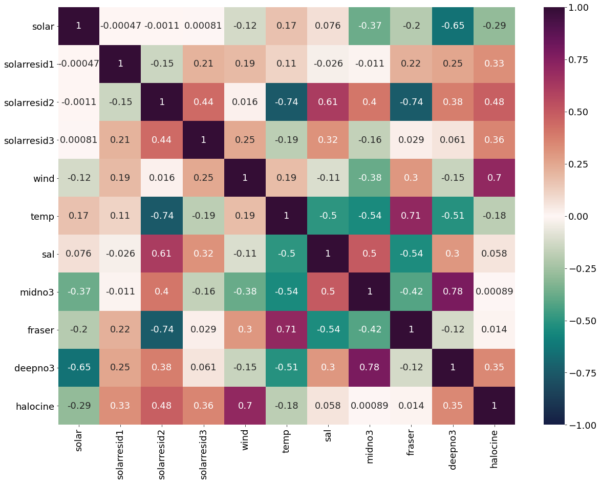
Correlation plots of solar radiation residuals
[17]:
#  residual calculations for each metric
solarresid1=list()
y,r2,m,b=bloomdrivers.reg_r2(solarmar,yearday1)
for ind,y in enumerate(yearday1):
    x=solarmar[ind]
    solarresid1.append(y-(m*x+b))

solarresid2=list()
y,r2,m,b=bloomdrivers.reg_r2(solarmar,yearday2)
for ind,y in enumerate(yearday2):
    x=solarmar[ind]
    solarresid2.append(y-(m*x+b))

solarresid3=list()
y,r2,m,b=bloomdrivers.reg_r2(solarmar,yearday3)
for ind,y in enumerate(yearday3):
    x=solarmar[ind]
    solarresid3.append(y-(m*x+b))
[18]:
dfsolar=pd.DataFrame({'solar':solarmar,'solarresid1':solarresid1,'solarresid2':solarresid2,'solarresid3':solarresid3,'wind':windmar,
                  'temp':tempmar,'sal':salmar,'midno3':midno3mar,'fraser':frasermar,'deepno3':deepno3mar,'halocine':halomar})
[19]:
plt.subplots(figsize=(20,15))
cm1=cmocean.cm.curl
sns.heatmap(dfsolar.corr(), annot = True,cmap=cm1,vmin=-1,vmax=1)
[19]:
<AxesSubplot:>
[20]:
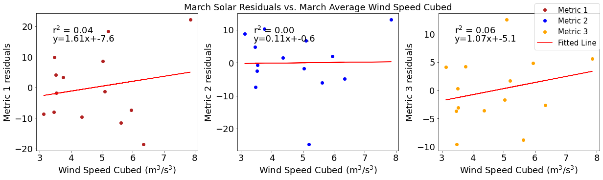
# ---------- wind ---------
fig4,ax4=plt.subplots(1,3,figsize=(17,5),constrained_layout=True)
ax4[0].plot(windmar,solarresid1,'o',color='firebrick',label='Metric 1')
ax4[0].set_xlabel('Wind Speed Cubed ($\mathregular{m^3}$/$\mathregular{s^3}$)')
ax4[0].set_ylabel('Metric 1 residuals')
y,r2,m,b=bloomdrivers.reg_r2(windmar,solarresid1)
ax4[0].plot(windmar, y, 'r')
ax4[0].text(0.1, 0.85, '$\mathregular{r^2}$ = %.2f'%r2, transform=ax4[0].transAxes)
ax4[0].text(0.1,0.78,f'y={round(m,2)}x+{round(b,1)}',horizontalalignment='left',verticalalignment='bottom',transform=ax4[0].transAxes)

ax4[1].plot(windmar,solarresid2,'o',color='b',label='Metric 2')
ax4[1].set_xlabel('Wind Speed Cubed ($\mathregular{m^3}$/$\mathregular{s^3}$)')
ax4[1].set_ylabel('Metric 2 residuals')
ax4[1].set_title('March Solar Residuals vs. March Average Wind Speed Cubed')
y,r2,m,b=bloomdrivers.reg_r2(windmar,solarresid2)
ax4[1].plot(windmar, y, 'r')
ax4[1].text(0.1, 0.85, '$\mathregular{r^2}$ = %.2f'%r2, transform=ax4[1].transAxes)
ax4[1].text(0.1,0.78,f'y={round(m,2)}x+{round(b,1)}',horizontalalignment='left',verticalalignment='bottom',transform=ax4[1].transAxes)

ax4[2].plot(windmar,solarresid3,'o',color='orange',label='Metric 3')
ax4[2].set_xlabel('Wind Speed Cubed ($\mathregular{m^3}$/$\mathregular{s^3}$)')
ax4[2].set_ylabel('Metric 3 residuals')
y,r2,m,b=bloomdrivers.reg_r2(windmar,solarresid3)
ax4[2].plot(windmar, y, 'r', label='Fitted Line')
ax4[2].text(0.1, 0.85, '$\mathregular{r^2}$ = %.2f'%r2, transform=ax4[2].transAxes)
ax4[2].text(0.1,0.78,f'y={round(m,2)}x+{round(b,1)}',horizontalalignment='left',verticalalignment='bottom',transform=ax4[2].transAxes)
fig4.legend()
[20]:
<matplotlib.legend.Legend at 0x7f0203e4ee50>
[21]:
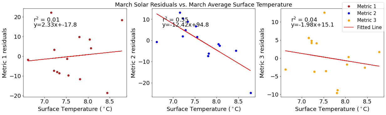
# ---------- Temperature ---------
fig4,ax4=plt.subplots(1,3,figsize=(17,5),constrained_layout=True)
ax4[0].plot(tempmar,solarresid1,'o',color='firebrick',label='Metric 1')
ax4[0].set_xlabel('Surface Temperature ($^\circ$C)')
ax4[0].set_ylabel('Metric 1 residuals')
y,r2,m,b=bloomdrivers.reg_r2(tempmar,solarresid1)
ax4[0].plot(tempmar, y, 'r')
ax4[0].text(0.1, 0.85, '$\mathregular{r^2}$ = %.2f'%r2, transform=ax4[0].transAxes)
ax4[0].text(0.1,0.78,f'y={round(m,2)}x+{round(b,1)}',horizontalalignment='left',verticalalignment='bottom',transform=ax4[0].transAxes)

ax4[1].plot(tempmar,solarresid2,'o',color='b',label='Metric 2')
ax4[1].set_xlabel('Surface Temperature ($^\circ$C)')
ax4[1].set_ylabel('Metric 2 residuals')
ax4[1].set_title('March Solar Residuals vs. March Average Surface Temperature')
y,r2,m,b=bloomdrivers.reg_r2(tempmar,solarresid2)
ax4[1].plot(tempmar, y, 'r')
ax4[1].text(0.1, 0.85, '$\mathregular{r^2}$ = %.2f'%r2, transform=ax4[1].transAxes)
ax4[1].text(0.1,0.78,f'y={round(m,2)}x+{round(b,1)}',horizontalalignment='left',verticalalignment='bottom',transform=ax4[1].transAxes)

ax4[2].plot(tempmar,solarresid3,'o',color='orange',label='Metric 3')
ax4[2].set_xlabel('Surface Temperature ($^\circ$C)')
ax4[2].set_ylabel('Metric 3 residuals')
y,r2,m,b=bloomdrivers.reg_r2(tempmar,solarresid3)
ax4[2].plot(tempmar, y, 'r', label='Fitted Line')
ax4[2].text(0.1, 0.85, '$\mathregular{r^2}$ = %.2f'%r2, transform=ax4[2].transAxes)
ax4[2].text(0.1,0.78,f'y={round(m,2)}x+{round(b,1)}',horizontalalignment='left',verticalalignment='bottom',transform=ax4[2].transAxes)
fig4.legend()
[21]:
<matplotlib.legend.Legend at 0x7f0203d8afa0>
[22]:
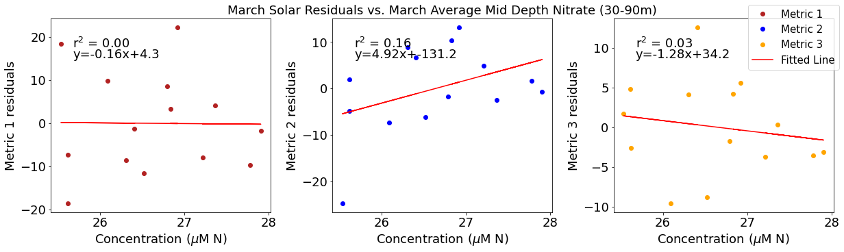
# ---------- Mid NO3 ---------
fig4,ax4=plt.subplots(1,3,figsize=(17,5),constrained_layout=True)
ax4[0].plot(midno3mar,solarresid1,'o',color='firebrick',label='Metric 1')
ax4[0].set_xlabel('Concentration ($\mu$M N)')
ax4[0].set_ylabel('Metric 1 residuals')
y,r2,m,b=bloomdrivers.reg_r2(midno3mar,solarresid1)
ax4[0].plot(midno3mar, y, 'r')
ax4[0].text(0.1, 0.85, '$\mathregular{r^2}$ = %.2f'%r2, transform=ax4[0].transAxes)
ax4[0].text(0.1,0.78,f'y={round(m,2)}x+{round(b,1)}',horizontalalignment='left',verticalalignment='bottom',transform=ax4[0].transAxes)

ax4[1].plot(midno3mar,solarresid2,'o',color='b',label='Metric 2')
ax4[1].set_xlabel('Concentration ($\mu$M N)')
ax4[1].set_ylabel('Metric 2 residuals')
ax4[1].set_title('March Solar Residuals vs. March Average Mid Depth Nitrate (30-90m)')
y,r2,m,b=bloomdrivers.reg_r2(midno3mar,solarresid2)
ax4[1].plot(midno3mar, y, 'r')
ax4[1].text(0.1, 0.85, '$\mathregular{r^2}$ = %.2f'%r2, transform=ax4[1].transAxes)
ax4[1].text(0.1,0.78,f'y={round(m,2)}x+{round(b,1)}',horizontalalignment='left',verticalalignment='bottom',transform=ax4[1].transAxes)

ax4[2].plot(midno3mar,solarresid3,'o',color='orange',label='Metric 3')
ax4[2].set_xlabel('Concentration ($\mu$M N)')
ax4[2].set_ylabel('Metric 3 residuals')
y,r2,m,b=bloomdrivers.reg_r2(midno3mar,solarresid3)
ax4[2].plot(midno3mar, y, 'r', label='Fitted Line')
ax4[2].text(0.1, 0.85, '$\mathregular{r^2}$ = %.2f'%r2, transform=ax4[2].transAxes)
ax4[2].text(0.1,0.78,f'y={round(m,2)}x+{round(b,1)}',horizontalalignment='left',verticalalignment='bottom',transform=ax4[2].transAxes)
fig4.legend()
[22]:
<matplotlib.legend.Legend at 0x7f0203c3a4c0>
[23]:
# ---------- Deep NO3 ---------
fig4,ax4=plt.subplots(1,3,figsize=(17,5),constrained_layout=True)
ax4[0].plot(deepno3mar,solarresid1,'o',color='firebrick',label='Metric 1')
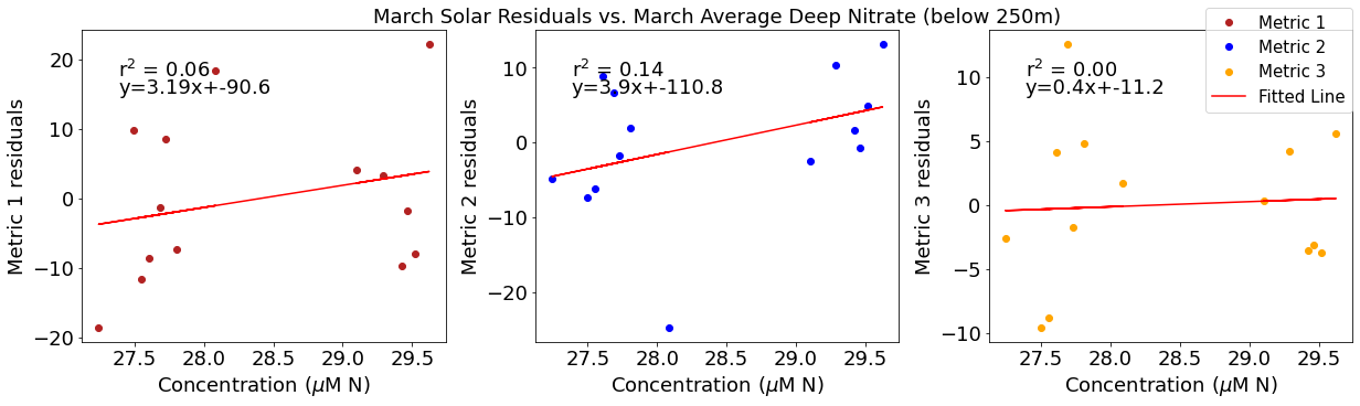
ax4[0].set_xlabel('Concentration ($\mu$M N)')
ax4[0].set_ylabel('Metric 1 residuals')
y,r2,m,b=bloomdrivers.reg_r2(deepno3mar,solarresid1)
ax4[0].plot(deepno3mar, y, 'r')
ax4[0].text(0.1, 0.85, '$\mathregular{r^2}$ = %.2f'%r2, transform=ax4[0].transAxes)
ax4[0].text(0.1,0.78,f'y={round(m,2)}x+{round(b,1)}',horizontalalignment='left',verticalalignment='bottom',transform=ax4[0].transAxes)
ax4[1].plot(deepno3mar,solarresid2,'o',color='b',label='Metric 2')
ax4[1].set_xlabel('Concentration ($\mu$M N)')
ax4[1].set_ylabel('Metric 2 residuals')
ax4[1].set_title('March Solar Residuals vs. March Average Deep Nitrate (below 250m)')
y,r2,m,b=bloomdrivers.reg_r2(deepno3mar,solarresid2)
ax4[1].plot(deepno3mar, y, 'r')
ax4[1].text(0.1, 0.85, '$\mathregular{r^2}$ = %.2f'%r2, transform=ax4[1].transAxes)
ax4[1].text(0.1,0.78,f'y={round(m,2)}x+{round(b,1)}',horizontalalignment='left',verticalalignment='bottom',transform=ax4[1].transAxes)
ax4[2].plot(deepno3mar,solarresid3,'o',color='orange',label='Metric 3')
ax4[2].set_xlabel('Concentration ($\mu$M N)')
ax4[2].set_ylabel('Metric 3 residuals')
y,r2,m,b=bloomdrivers.reg_r2(deepno3mar,solarresid3)
ax4[2].plot(deepno3mar, y, 'r', label='Fitted Line')
ax4[2].text(0.1, 0.85, '$\mathregular{r^2}$ = %.2f'%r2, transform=ax4[2].transAxes)
ax4[2].text(0.1,0.78,f'y={round(m,2)}x+{round(b,1)}',horizontalalignment='left',verticalalignment='bottom',transform=ax4[2].transAxes)
fig4.legend()
[23]:
<matplotlib.legend.Legend at 0x7f0203adbee0>
[24]:
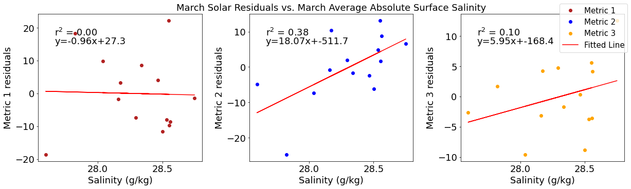
# ---------- Salinity ---------
fig4,ax4=plt.subplots(1,3,figsize=(17,5),constrained_layout=True)
ax4[0].plot(salmar,solarresid1,'o',color='firebrick',label='Metric 1')
ax4[0].set_xlabel('Salinity (g/kg)')
ax4[0].set_ylabel('Metric 1 residuals')
y,r2,m,b=bloomdrivers.reg_r2(salmar,solarresid1)
ax4[0].plot(salmar, y, 'r')
ax4[0].text(0.1, 0.85, '$\mathregular{r^2}$ = %.2f'%r2, transform=ax4[0].transAxes)
ax4[0].text(0.1,0.78,f'y={round(m,2)}x+{round(b,1)}',horizontalalignment='left',verticalalignment='bottom',transform=ax4[0].transAxes)

ax4[1].plot(salmar,solarresid2,'o',color='b',label='Metric 2')
ax4[1].set_xlabel('Salinity (g/kg)')
ax4[1].set_ylabel('Metric 2 residuals')
ax4[1].set_title('March Solar Residuals vs. March Average Absolute Surface Salinity')
y,r2,m,b=bloomdrivers.reg_r2(salmar,solarresid2)
ax4[1].plot(salmar, y, 'r')
ax4[1].text(0.1, 0.85, '$\mathregular{r^2}$ = %.2f'%r2, transform=ax4[1].transAxes)
ax4[1].text(0.1,0.78,f'y={round(m,2)}x+{round(b,1)}',horizontalalignment='left',verticalalignment='bottom',transform=ax4[1].transAxes)

ax4[2].plot(salmar,solarresid3,'o',color='orange',label='Metric 3')
ax4[2].set_xlabel('Salinity (g/kg)')
ax4[2].set_ylabel('Metric 3 residuals')
y,r2,m,b=bloomdrivers.reg_r2(salmar,solarresid3)
ax4[2].plot(salmar, y, 'r', label='Fitted Line')
ax4[2].text(0.1, 0.85, '$\mathregular{r^2}$ = %.2f'%r2, transform=ax4[2].transAxes)
ax4[2].text(0.1,0.78,f'y={round(m,2)}x+{round(b,1)}',horizontalalignment='left',verticalalignment='bottom',transform=ax4[2].transAxes)
fig4.legend()
[24]:
<matplotlib.legend.Legend at 0x7f0203983e80>
[25]:
# ---------- Fraser ---------
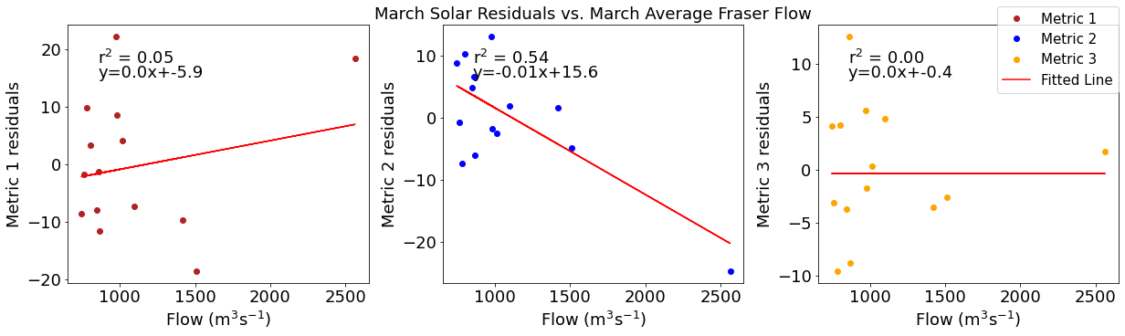
fig4,ax4=plt.subplots(1,3,figsize=(17,5),constrained_layout=True)
ax4[0].plot(frasermar,solarresid1,'o',color='firebrick',label='Metric 1')
ax4[0].set_xlabel('Flow (m$^3$s$^{-1}$)')
ax4[0].set_ylabel('Metric 1 residuals')
y,r2,m,b=bloomdrivers.reg_r2(frasermar,solarresid1)
ax4[0].plot(frasermar, y, 'r')
ax4[0].text(0.1, 0.85, '$\mathregular{r^2}$ = %.2f'%r2, transform=ax4[0].transAxes)
ax4[0].text(0.1,0.78,f'y={round(m,2)}x+{round(b,1)}',horizontalalignment='left',verticalalignment='bottom',transform=ax4[0].transAxes)
ax4[1].plot(frasermar,solarresid2,'o',color='b',label='Metric 2')
ax4[1].set_xlabel('Flow (m$^3$s$^{-1}$)')
ax4[1].set_ylabel('Metric 2 residuals')
ax4[1].set_title('March Solar Residuals vs. March Average Fraser Flow')
y,r2,m,b=bloomdrivers.reg_r2(frasermar,solarresid2)
ax4[1].plot(frasermar, y, 'r')
ax4[1].text(0.1, 0.85, '$\mathregular{r^2}$ = %.2f'%r2, transform=ax4[1].transAxes)
ax4[1].text(0.1,0.78,f'y={round(m,2)}x+{round(b,1)}',horizontalalignment='left',verticalalignment='bottom',transform=ax4[1].transAxes)
ax4[2].plot(frasermar,solarresid3,'o',color='orange',label='Metric 3')
ax4[2].set_xlabel('Flow (m$^3$s$^{-1}$)')
ax4[2].set_ylabel('Metric 3 residuals')
y,r2,m,b=bloomdrivers.reg_r2(frasermar,solarresid3)
ax4[2].plot(frasermar, y, 'r', label='Fitted Line')
ax4[2].text(0.1, 0.85, '$\mathregular{r^2}$ = %.2f'%r2, transform=ax4[2].transAxes)
ax4[2].text(0.1,0.78,f'y={round(m,2)}x+{round(b,1)}',horizontalalignment='left',verticalalignment='bottom',transform=ax4[2].transAxes)
fig4.legend()
[25]:
<matplotlib.legend.Legend at 0x7f02038af1c0>
[26]:
# ---------- Halocline ---------
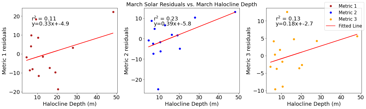
fig4,ax4=plt.subplots(1,3,figsize=(17,5),constrained_layout=True)
ax4[0].plot(halomar,solarresid1,'o',color='firebrick',label='Metric 1')
ax4[0].set_xlabel('Halocline Depth (m)')
ax4[0].set_ylabel('Metric 1 residuals')
y,r2,m,b=bloomdrivers.reg_r2(halomar,solarresid1)
ax4[0].plot(halomar, y, 'r')
ax4[0].text(0.1, 0.85, '$\mathregular{r^2}$ = %.2f'%r2, transform=ax4[0].transAxes)
ax4[0].text(0.1,0.78,f'y={round(m,2)}x+{round(b,1)}',horizontalalignment='left',verticalalignment='bottom',transform=ax4[0].transAxes)
ax4[1].plot(halomar,solarresid2,'o',color='b',label='Metric 2')
ax4[1].set_xlabel('Halocline Depth (m)')
ax4[1].set_ylabel('Metric 2 residuals')
ax4[1].set_title('March Solar Residuals vs. March Halocline Depth')
y,r2,m,b=bloomdrivers.reg_r2(halomar,solarresid2)
ax4[1].plot(halomar, y, 'r')
ax4[1].text(0.1, 0.85, '$\mathregular{r^2}$ = %.2f'%r2, transform=ax4[1].transAxes)
ax4[1].text(0.1,0.78,f'y={round(m,2)}x+{round(b,1)}',horizontalalignment='left',verticalalignment='bottom',transform=ax4[1].transAxes)
ax4[2].plot(halomar,solarresid3,'o',color='orange',label='Metric 3')
ax4[2].set_xlabel('Halocline Depth (m)')
ax4[2].set_ylabel('Metric 3 residuals')
y,r2,m,b=bloomdrivers.reg_r2(halomar,solarresid3)
ax4[2].plot(halomar, y, 'r', label='Fitted Line')
ax4[2].text(0.1, 0.85, '$\mathregular{r^2}$ = %.2f'%r2, transform=ax4[2].transAxes)
ax4[2].text(0.1,0.78,f'y={round(m,2)}x+{round(b,1)}',horizontalalignment='left',verticalalignment='bottom',transform=ax4[2].transAxes)
fig4.legend()
[26]:
<matplotlib.legend.Legend at 0x7f020374f0a0>
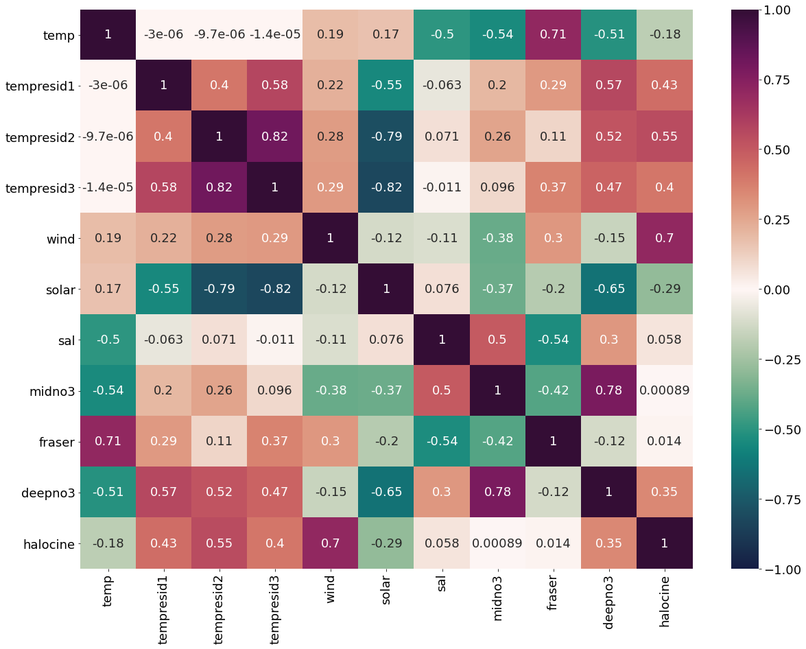
Correlation plots of temperature residuals
[27]:
#  residual calculations for each metric
tempresid1=list()
y,r2,m,b=bloomdrivers.reg_r2(tempmar,yearday1)
for ind,y in enumerate(yearday1):
    x=tempmar[ind]
    tempresid1.append(y-(m*x+b))

tempresid2=list()
y,r2,m,b=bloomdrivers.reg_r2(tempmar,yearday2)
for ind,y in enumerate(yearday2):
    x=tempmar[ind]
    tempresid2.append(y-(m*x+b))

tempresid3=list()
y,r2,m,b=bloomdrivers.reg_r2(tempmar,yearday3)
for ind,y in enumerate(yearday3):
    x=tempmar[ind]
    tempresid3.append(y-(m*x+b))
[28]:
dftemp=pd.DataFrame({'temp':tempmar,'tempresid1':tempresid1,'tempresid2':tempresid2,'tempresid3':tempresid3,'wind':windmar,'solar':solarmar,
                  'sal':salmar,'midno3':midno3mar,'fraser':frasermar,'deepno3':deepno3mar,'halocine':halomar})
[29]:
plt.subplots(figsize=(20,15))
cm1=cmocean.cm.curl
sns.heatmap(dftemp.corr(), annot = True,cmap=cm1,vmin=-1,vmax=1)
[29]:
<AxesSubplot:>
[30]:
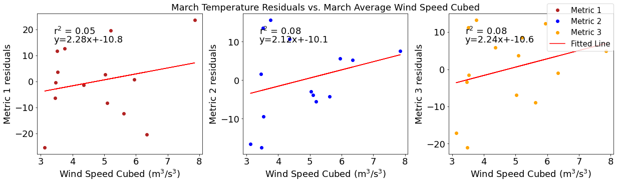
# ---------- wind ---------
fig4,ax4=plt.subplots(1,3,figsize=(17,5),constrained_layout=True)
ax4[0].plot(windmar,tempresid1,'o',color='firebrick',label='Metric 1')
ax4[0].set_xlabel('Wind Speed Cubed ($\mathregular{m^3}$/$\mathregular{s^3}$)')
ax4[0].set_ylabel('Metric 1 residuals')
y,r2,m,b=bloomdrivers.reg_r2(windmar,tempresid1)
ax4[0].plot(windmar, y, 'r')
ax4[0].text(0.1, 0.85, '$\mathregular{r^2}$ = %.2f'%r2, transform=ax4[0].transAxes)
ax4[0].text(0.1,0.78,f'y={round(m,2)}x+{round(b,1)}',horizontalalignment='left',verticalalignment='bottom',transform=ax4[0].transAxes)

ax4[1].plot(windmar,tempresid2,'o',color='b',label='Metric 2')
ax4[1].set_xlabel('Wind Speed Cubed ($\mathregular{m^3}$/$\mathregular{s^3}$)')
ax4[1].set_ylabel('Metric 2 residuals')
ax4[1].set_title('March Temperature Residuals vs. March Average Wind Speed Cubed')
y,r2,m,b=bloomdrivers.reg_r2(windmar,tempresid2)
ax4[1].plot(windmar, y, 'r')
ax4[1].text(0.1, 0.85, '$\mathregular{r^2}$ = %.2f'%r2, transform=ax4[1].transAxes)
ax4[1].text(0.1,0.78,f'y={round(m,2)}x+{round(b,1)}',horizontalalignment='left',verticalalignment='bottom',transform=ax4[1].transAxes)

ax4[2].plot(windmar,tempresid3,'o',color='orange',label='Metric 3')
ax4[2].set_xlabel('Wind Speed Cubed ($\mathregular{m^3}$/$\mathregular{s^3}$)')
ax4[2].set_ylabel('Metric 3 residuals')
y,r2,m,b=bloomdrivers.reg_r2(windmar,tempresid3)
ax4[2].plot(windmar, y, 'r', label='Fitted Line')
ax4[2].text(0.1, 0.85, '$\mathregular{r^2}$ = %.2f'%r2, transform=ax4[2].transAxes)
ax4[2].text(0.1,0.78,f'y={round(m,2)}x+{round(b,1)}',horizontalalignment='left',verticalalignment='bottom',transform=ax4[2].transAxes)
fig4.legend()
[30]:
<matplotlib.legend.Legend at 0x7f02035653a0>
[31]:
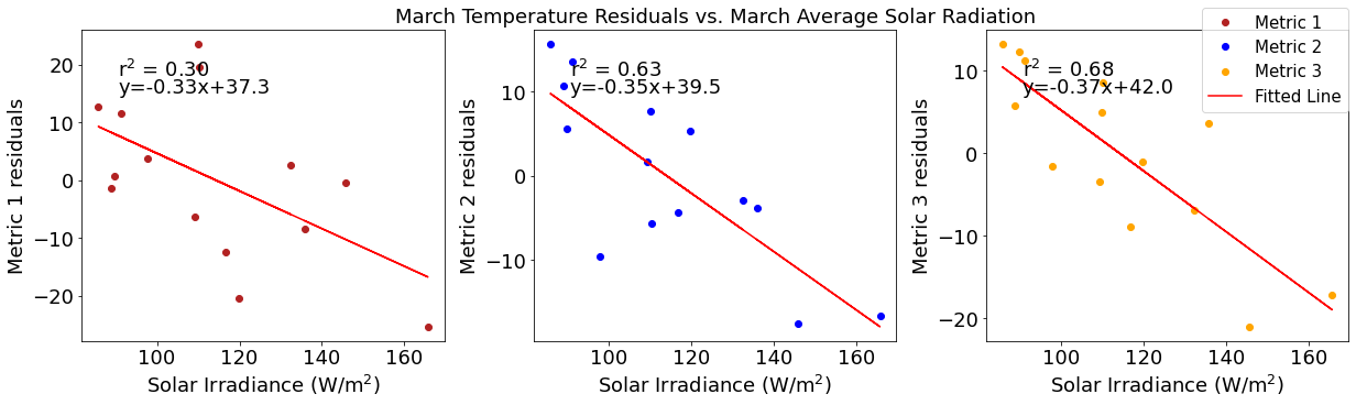
# ---------- Solar ---------
fig4,ax4=plt.subplots(1,3,figsize=(17,5),constrained_layout=True)
ax4[0].plot(solarmar,tempresid1,'o',color='firebrick',label='Metric 1')
ax4[0].set_xlabel('Solar Irradiance (W/$\mathregular{m^2}$)')
ax4[0].set_ylabel('Metric 1 residuals')
y,r2,m,b=bloomdrivers.reg_r2(solarmar,tempresid1)
ax4[0].plot(solarmar, y, 'r')
ax4[0].text(0.1, 0.85, '$\mathregular{r^2}$ = %.2f'%r2, transform=ax4[0].transAxes)
ax4[0].text(0.1,0.78,f'y={round(m,2)}x+{round(b,1)}',horizontalalignment='left',verticalalignment='bottom',transform=ax4[0].transAxes)

ax4[1].plot(solarmar,tempresid2,'o',color='b',label='Metric 2')
ax4[1].set_xlabel('Solar Irradiance (W/$\mathregular{m^2}$)')
ax4[1].set_ylabel('Metric 2 residuals')
ax4[1].set_title('March Temperature Residuals vs. March Average Solar Radiation')
y,r2,m,b=bloomdrivers.reg_r2(solarmar,tempresid2)
ax4[1].plot(solarmar, y, 'r')
ax4[1].text(0.1, 0.85, '$\mathregular{r^2}$ = %.2f'%r2, transform=ax4[1].transAxes)
ax4[1].text(0.1,0.78,f'y={round(m,2)}x+{round(b,1)}',horizontalalignment='left',verticalalignment='bottom',transform=ax4[1].transAxes)

ax4[2].plot(solarmar,tempresid3,'o',color='orange',label='Metric 3')
ax4[2].set_xlabel('Solar Irradiance (W/$\mathregular{m^2}$)')
ax4[2].set_ylabel('Metric 3 residuals')
y,r2,m,b=bloomdrivers.reg_r2(solarmar,tempresid3)
ax4[2].plot(solarmar, y, 'r', label='Fitted Line')
ax4[2].text(0.1, 0.85, '$\mathregular{r^2}$ = %.2f'%r2, transform=ax4[2].transAxes)
ax4[2].text(0.1,0.78,f'y={round(m,2)}x+{round(b,1)}',horizontalalignment='left',verticalalignment='bottom',transform=ax4[2].transAxes)
fig4.legend()
[31]:
<matplotlib.legend.Legend at 0x7f020341a460>
[32]:
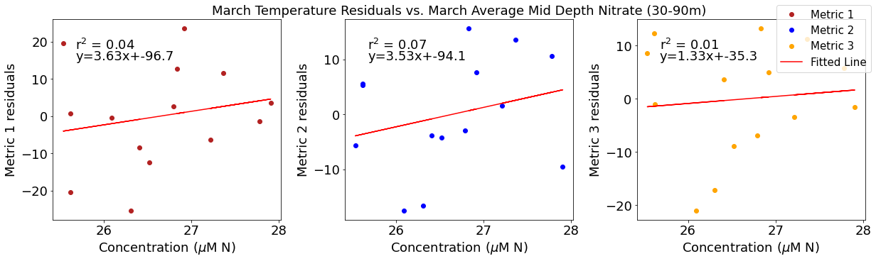
# ---------- Mid NO3 ---------
fig4,ax4=plt.subplots(1,3,figsize=(17,5),constrained_layout=True)
ax4[0].plot(midno3mar,tempresid1,'o',color='firebrick',label='Metric 1')
ax4[0].set_xlabel('Concentration ($\mu$M N)')
ax4[0].set_ylabel('Metric 1 residuals')
y,r2,m,b=bloomdrivers.reg_r2(midno3mar,tempresid1)
ax4[0].plot(midno3mar, y, 'r')
ax4[0].text(0.1, 0.85, '$\mathregular{r^2}$ = %.2f'%r2, transform=ax4[0].transAxes)
ax4[0].text(0.1,0.78,f'y={round(m,2)}x+{round(b,1)}',horizontalalignment='left',verticalalignment='bottom',transform=ax4[0].transAxes)

ax4[1].plot(midno3mar,tempresid2,'o',color='b',label='Metric 2')
ax4[1].set_xlabel('Concentration ($\mu$M N)')
ax4[1].set_ylabel('Metric 2 residuals')
ax4[1].set_title('March Temperature Residuals vs. March Average Mid Depth Nitrate (30-90m)')
y,r2,m,b=bloomdrivers.reg_r2(midno3mar,tempresid2)
ax4[1].plot(midno3mar, y, 'r')
ax4[1].text(0.1, 0.85, '$\mathregular{r^2}$ = %.2f'%r2, transform=ax4[1].transAxes)
ax4[1].text(0.1,0.78,f'y={round(m,2)}x+{round(b,1)}',horizontalalignment='left',verticalalignment='bottom',transform=ax4[1].transAxes)

ax4[2].plot(midno3mar,tempresid3,'o',color='orange',label='Metric 3')
ax4[2].set_xlabel('Concentration ($\mu$M N)')
ax4[2].set_ylabel('Metric 3 residuals')
y,r2,m,b=bloomdrivers.reg_r2(midno3mar,tempresid3)
ax4[2].plot(midno3mar, y, 'r', label='Fitted Line')
ax4[2].text(0.1, 0.85, '$\mathregular{r^2}$ = %.2f'%r2, transform=ax4[2].transAxes)
ax4[2].text(0.1,0.78,f'y={round(m,2)}x+{round(b,1)}',horizontalalignment='left',verticalalignment='bottom',transform=ax4[2].transAxes)
fig4.legend()
[32]:
<matplotlib.legend.Legend at 0x7f0203330e20>
[33]:
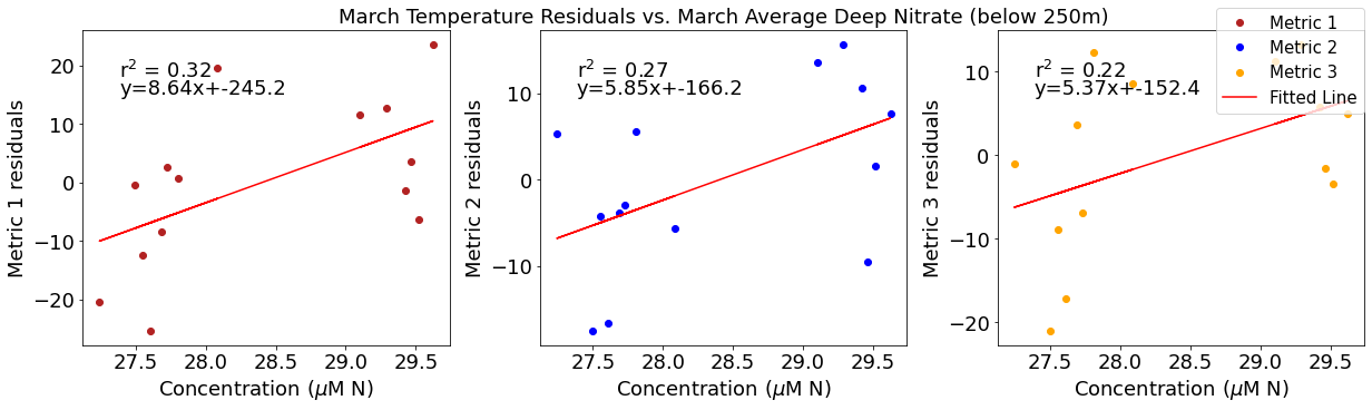
# ---------- Deep NO3 ---------
fig4,ax4=plt.subplots(1,3,figsize=(17,5),constrained_layout=True)
ax4[0].plot(deepno3mar,tempresid1,'o',color='firebrick',label='Metric 1')
ax4[0].set_xlabel('Concentration ($\mu$M N)')
ax4[0].set_ylabel('Metric 1 residuals')
y,r2,m,b=bloomdrivers.reg_r2(deepno3mar,tempresid1)
ax4[0].plot(deepno3mar, y, 'r')
ax4[0].text(0.1, 0.85, '$\mathregular{r^2}$ = %.2f'%r2, transform=ax4[0].transAxes)
ax4[0].text(0.1,0.78,f'y={round(m,2)}x+{round(b,1)}',horizontalalignment='left',verticalalignment='bottom',transform=ax4[0].transAxes)

ax4[1].plot(deepno3mar,tempresid2,'o',color='b',label='Metric 2')
ax4[1].set_xlabel('Concentration ($\mu$M N)')
ax4[1].set_ylabel('Metric 2 residuals')
ax4[1].set_title('March Temperature Residuals vs. March Average Deep Nitrate (below 250m)')
y,r2,m,b=bloomdrivers.reg_r2(deepno3mar,tempresid2)
ax4[1].plot(deepno3mar, y, 'r')
ax4[1].text(0.1, 0.85, '$\mathregular{r^2}$ = %.2f'%r2, transform=ax4[1].transAxes)
ax4[1].text(0.1,0.78,f'y={round(m,2)}x+{round(b,1)}',horizontalalignment='left',verticalalignment='bottom',transform=ax4[1].transAxes)

ax4[2].plot(deepno3mar,tempresid3,'o',color='orange',label='Metric 3')
ax4[2].set_xlabel('Concentration ($\mu$M N)')
ax4[2].set_ylabel('Metric 3 residuals')
y,r2,m,b=bloomdrivers.reg_r2(deepno3mar,tempresid3)
ax4[2].plot(deepno3mar, y, 'r', label='Fitted Line')
ax4[2].text(0.1, 0.85, '$\mathregular{r^2}$ = %.2f'%r2, transform=ax4[2].transAxes)
ax4[2].text(0.1,0.78,f'y={round(m,2)}x+{round(b,1)}',horizontalalignment='left',verticalalignment='bottom',transform=ax4[2].transAxes)
fig4.legend()
[33]:
<matplotlib.legend.Legend at 0x7f02031c5d90>
[34]:
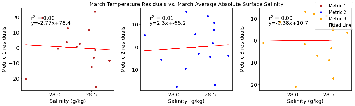
# ---------- Salinity ---------
fig4,ax4=plt.subplots(1,3,figsize=(17,5),constrained_layout=True)
ax4[0].plot(salmar,tempresid1,'o',color='firebrick',label='Metric 1')
ax4[0].set_xlabel('Salinity (g/kg)')
ax4[0].set_ylabel('Metric 1 residuals')
y,r2,m,b=bloomdrivers.reg_r2(salmar,tempresid1)
ax4[0].plot(salmar, y, 'r')
ax4[0].text(0.1, 0.85, '$\mathregular{r^2}$ = %.2f'%r2, transform=ax4[0].transAxes)
ax4[0].text(0.1,0.78,f'y={round(m,2)}x+{round(b,1)}',horizontalalignment='left',verticalalignment='bottom',transform=ax4[0].transAxes)

ax4[1].plot(salmar,tempresid2,'o',color='b',label='Metric 2')
ax4[1].set_xlabel('Salinity (g/kg)')
ax4[1].set_ylabel('Metric 2 residuals')
ax4[1].set_title('March Temperature Residuals vs. March Average Absolute Surface Salinity')
y,r2,m,b=bloomdrivers.reg_r2(salmar,tempresid2)
ax4[1].plot(salmar, y, 'r')
ax4[1].text(0.1, 0.85, '$\mathregular{r^2}$ = %.2f'%r2, transform=ax4[1].transAxes)
ax4[1].text(0.1,0.78,f'y={round(m,2)}x+{round(b,1)}',horizontalalignment='left',verticalalignment='bottom',transform=ax4[1].transAxes)

ax4[2].plot(salmar,tempresid3,'o',color='orange',label='Metric 3')
ax4[2].set_xlabel('Salinity (g/kg)')
ax4[2].set_ylabel('Metric 3 residuals')
y,r2,m,b=bloomdrivers.reg_r2(salmar,tempresid3)
ax4[2].plot(salmar, y, 'r', label='Fitted Line')
ax4[2].text(0.1, 0.85, '$\mathregular{r^2}$ = %.2f'%r2, transform=ax4[2].transAxes)
ax4[2].text(0.1,0.78,f'y={round(m,2)}x+{round(b,1)}',horizontalalignment='left',verticalalignment='bottom',transform=ax4[2].transAxes)
fig4.legend()
[34]:
<matplotlib.legend.Legend at 0x7f02030e2c40>
[35]:
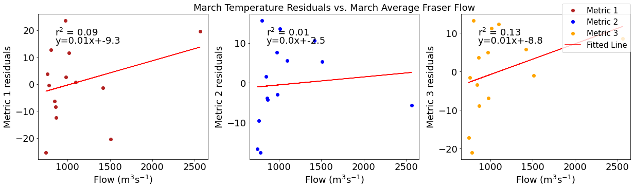
# ---------- Fraser ---------
fig4,ax4=plt.subplots(1,3,figsize=(17,5),constrained_layout=True)
ax4[0].plot(frasermar,tempresid1,'o',color='firebrick',label='Metric 1')
ax4[0].set_xlabel('Flow (m$^3$s$^{-1}$)')
ax4[0].set_ylabel('Metric 1 residuals')
y,r2,m,b=bloomdrivers.reg_r2(frasermar,tempresid1)
ax4[0].plot(frasermar, y, 'r')
ax4[0].text(0.1, 0.85, '$\mathregular{r^2}$ = %.2f'%r2, transform=ax4[0].transAxes)
ax4[0].text(0.1,0.78,f'y={round(m,2)}x+{round(b,1)}',horizontalalignment='left',verticalalignment='bottom',transform=ax4[0].transAxes)

ax4[1].plot(frasermar,tempresid2,'o',color='b',label='Metric 2')
ax4[1].set_xlabel('Flow (m$^3$s$^{-1}$)')
ax4[1].set_ylabel('Metric 2 residuals')
ax4[1].set_title('March Temperature Residuals vs. March Average Fraser Flow')
y,r2,m,b=bloomdrivers.reg_r2(frasermar,tempresid2)
ax4[1].plot(frasermar, y, 'r')
ax4[1].text(0.1, 0.85, '$\mathregular{r^2}$ = %.2f'%r2, transform=ax4[1].transAxes)
ax4[1].text(0.1,0.78,f'y={round(m,2)}x+{round(b,1)}',horizontalalignment='left',verticalalignment='bottom',transform=ax4[1].transAxes)

ax4[2].plot(frasermar,tempresid3,'o',color='orange',label='Metric 3')
ax4[2].set_xlabel('Flow (m$^3$s$^{-1}$)')
ax4[2].set_ylabel('Metric 3 residuals')
y,r2,m,b=bloomdrivers.reg_r2(frasermar,tempresid3)
ax4[2].plot(frasermar, y, 'r', label='Fitted Line')
ax4[2].text(0.1, 0.85, '$\mathregular{r^2}$ = %.2f'%r2, transform=ax4[2].transAxes)
ax4[2].text(0.1,0.78,f'y={round(m,2)}x+{round(b,1)}',horizontalalignment='left',verticalalignment='bottom',transform=ax4[2].transAxes)
fig4.legend()
[35]:
<matplotlib.legend.Legend at 0x7f0202feb5b0>
[36]:
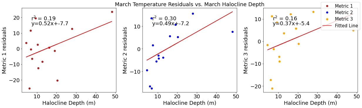
# ---------- Halocline ---------
fig4,ax4=plt.subplots(1,3,figsize=(17,5),constrained_layout=True)
ax4[0].plot(halomar,tempresid1,'o',color='firebrick',label='Metric 1')
ax4[0].set_xlabel('Halocline Depth (m)')
ax4[0].set_ylabel('Metric 1 residuals')
y,r2,m,b=bloomdrivers.reg_r2(halomar,tempresid1)
ax4[0].plot(halomar, y, 'r')
ax4[0].text(0.1, 0.85, '$\mathregular{r^2}$ = %.2f'%r2, transform=ax4[0].transAxes)
ax4[0].text(0.1,0.78,f'y={round(m,2)}x+{round(b,1)}',horizontalalignment='left',verticalalignment='bottom',transform=ax4[0].transAxes)

ax4[1].plot(halomar,tempresid2,'o',color='b',label='Metric 2')
ax4[1].set_xlabel('Halocline Depth (m)')
ax4[1].set_ylabel('Metric 2 residuals')
ax4[1].set_title('March Temperature Residuals vs. March Halocline Depth')
y,r2,m,b=bloomdrivers.reg_r2(halomar,tempresid2)
ax4[1].plot(halomar, y, 'r')
ax4[1].text(0.1, 0.85, '$\mathregular{r^2}$ = %.2f'%r2, transform=ax4[1].transAxes)
ax4[1].text(0.1,0.78,f'y={round(m,2)}x+{round(b,1)}',horizontalalignment='left',verticalalignment='bottom',transform=ax4[1].transAxes)

ax4[2].plot(halomar,tempresid3,'o',color='orange',label='Metric 3')
ax4[2].set_xlabel('Halocline Depth (m)')
ax4[2].set_ylabel('Metric 3 residuals')
y,r2,m,b=bloomdrivers.reg_r2(halomar,tempresid3)
ax4[2].plot(halomar, y, 'r', label='Fitted Line')
ax4[2].text(0.1, 0.85, '$\mathregular{r^2}$ = %.2f'%r2, transform=ax4[2].transAxes)
ax4[2].text(0.1,0.78,f'y={round(m,2)}x+{round(b,1)}',horizontalalignment='left',verticalalignment='bottom',transform=ax4[2].transAxes)
fig4.legend()
[36]:
<matplotlib.legend.Legend at 0x7f0202ef25e0>
Correlation plots of salinity residuals
[37]:
#  residual calculations for each metric
salresid1=list()
y,r2,m,b=bloomdrivers.reg_r2(salmar,yearday1)
for ind,y in enumerate(yearday1):
    x=salmar[ind]
    salresid1.append(y-(m*x+b))

salresid2=list()
y,r2,m,b=bloomdrivers.reg_r2(salmar,yearday2)
for ind,y in enumerate(yearday2):
    x=salmar[ind]
    salresid2.append(y-(m*x+b))

salresid3=list()
y,r2,m,b=bloomdrivers.reg_r2(salmar,yearday3)
for ind,y in enumerate(yearday3):
    x=salmar[ind]
    salresid3.append(y-(m*x+b))
[38]:
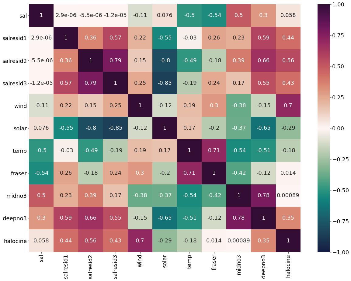
dfsal=pd.DataFrame({'sal':salmar,'salresid1':salresid1,'salresid2':salresid2,'salresid3':salresid3,'wind':windmar,'solar':solarmar,
                    'temp':tempmar,'fraser':frasermar,'midno3':midno3mar,'deepno3':deepno3mar,'halocine':halomar})
[39]:
plt.subplots(figsize=(20,15))
cm1=cmocean.cm.curl
sns.heatmap(dfsal.corr(), annot = True,cmap=cm1,vmin=-1,vmax=1)
[39]:
<AxesSubplot:>
[40]:
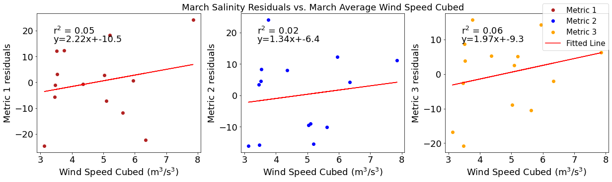
# ---------- wind ---------
fig4,ax4=plt.subplots(1,3,figsize=(17,5),constrained_layout=True)
ax4[0].plot(windmar,salresid1,'o',color='firebrick',label='Metric 1')
ax4[0].set_xlabel('Wind Speed Cubed ($\mathregular{m^3}$/$\mathregular{s^3}$)')
ax4[0].set_ylabel('Metric 1 residuals')
y,r2,m,b=bloomdrivers.reg_r2(windmar,salresid1)
ax4[0].plot(windmar, y, 'r')
ax4[0].text(0.1, 0.85, '$\mathregular{r^2}$ = %.2f'%r2, transform=ax4[0].transAxes)
ax4[0].text(0.1,0.78,f'y={round(m,2)}x+{round(b,1)}',horizontalalignment='left',verticalalignment='bottom',transform=ax4[0].transAxes)

ax4[1].plot(windmar,salresid2,'o',color='b',label='Metric 2')
ax4[1].set_xlabel('Wind Speed Cubed ($\mathregular{m^3}$/$\mathregular{s^3}$)')
ax4[1].set_ylabel('Metric 2 residuals')
ax4[1].set_title('March Salinity Residuals vs. March Average Wind Speed Cubed')
y,r2,m,b=bloomdrivers.reg_r2(windmar,salresid2)
ax4[1].plot(windmar, y, 'r')
ax4[1].text(0.1, 0.85, '$\mathregular{r^2}$ = %.2f'%r2, transform=ax4[1].transAxes)
ax4[1].text(0.1,0.78,f'y={round(m,2)}x+{round(b,1)}',horizontalalignment='left',verticalalignment='bottom',transform=ax4[1].transAxes)

ax4[2].plot(windmar,salresid3,'o',color='orange',label='Metric 3')
ax4[2].set_xlabel('Wind Speed Cubed ($\mathregular{m^3}$/$\mathregular{s^3}$)')
ax4[2].set_ylabel('Metric 3 residuals')
y,r2,m,b=bloomdrivers.reg_r2(windmar,salresid3)
ax4[2].plot(windmar, y, 'r', label='Fitted Line')
ax4[2].text(0.1, 0.85, '$\mathregular{r^2}$ = %.2f'%r2, transform=ax4[2].transAxes)
ax4[2].text(0.1,0.78,f'y={round(m,2)}x+{round(b,1)}',horizontalalignment='left',verticalalignment='bottom',transform=ax4[2].transAxes)
fig4.legend()
[40]:
<matplotlib.legend.Legend at 0x7f0202c16af0>
[41]:
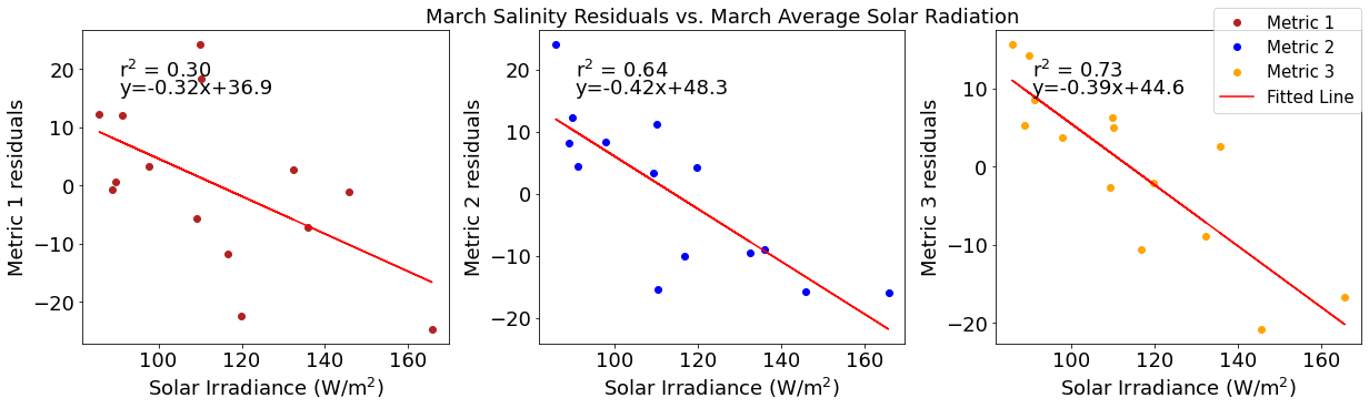
# ---------- Solar ---------
fig4,ax4=plt.subplots(1,3,figsize=(17,5),constrained_layout=True)
ax4[0].plot(solarmar,salresid1,'o',color='firebrick',label='Metric 1')
ax4[0].set_xlabel('Solar Irradiance (W/$\mathregular{m^2}$)')
ax4[0].set_ylabel('Metric 1 residuals')
y,r2,m,b=bloomdrivers.reg_r2(solarmar,salresid1)
ax4[0].plot(solarmar, y, 'r')
ax4[0].text(0.1, 0.85, '$\mathregular{r^2}$ = %.2f'%r2, transform=ax4[0].transAxes)
ax4[0].text(0.1,0.78,f'y={round(m,2)}x+{round(b,1)}',horizontalalignment='left',verticalalignment='bottom',transform=ax4[0].transAxes)

ax4[1].plot(solarmar,salresid2,'o',color='b',label='Metric 2')
ax4[1].set_xlabel('Solar Irradiance (W/$\mathregular{m^2}$)')
ax4[1].set_ylabel('Metric 2 residuals')
ax4[1].set_title('March Salinity Residuals vs. March Average Solar Radiation')
y,r2,m,b=bloomdrivers.reg_r2(solarmar,salresid2)
ax4[1].plot(solarmar, y, 'r')
ax4[1].text(0.1, 0.85, '$\mathregular{r^2}$ = %.2f'%r2, transform=ax4[1].transAxes)
ax4[1].text(0.1,0.78,f'y={round(m,2)}x+{round(b,1)}',horizontalalignment='left',verticalalignment='bottom',transform=ax4[1].transAxes)

ax4[2].plot(solarmar,salresid3,'o',color='orange',label='Metric 3')
ax4[2].set_xlabel('Solar Irradiance (W/$\mathregular{m^2}$)')
ax4[2].set_ylabel('Metric 3 residuals')
y,r2,m,b=bloomdrivers.reg_r2(solarmar,salresid3)
ax4[2].plot(solarmar, y, 'r', label='Fitted Line')
ax4[2].text(0.1, 0.85, '$\mathregular{r^2}$ = %.2f'%r2, transform=ax4[2].transAxes)
ax4[2].text(0.1,0.78,f'y={round(m,2)}x+{round(b,1)}',horizontalalignment='left',verticalalignment='bottom',transform=ax4[2].transAxes)
fig4.legend()
[41]:
<matplotlib.legend.Legend at 0x7f0202b9fa00>
[42]:
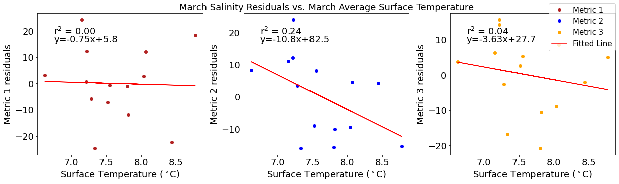
# ---------- Temperature ---------
fig4,ax4=plt.subplots(1,3,figsize=(17,5),constrained_layout=True)
ax4[0].plot(tempmar,salresid1,'o',color='firebrick',label='Metric 1')
ax4[0].set_xlabel('Surface Temperature ($^\circ$C)')
ax4[0].set_ylabel('Metric 1 residuals')
y,r2,m,b=bloomdrivers.reg_r2(tempmar,salresid1)
ax4[0].plot(tempmar, y, 'r')
ax4[0].text(0.1, 0.85, '$\mathregular{r^2}$ = %.2f'%r2, transform=ax4[0].transAxes)
ax4[0].text(0.1,0.78,f'y={round(m,2)}x+{round(b,1)}',horizontalalignment='left',verticalalignment='bottom',transform=ax4[0].transAxes)

ax4[1].plot(tempmar,salresid2,'o',color='b',label='Metric 2')
ax4[1].set_xlabel('Surface Temperature ($^\circ$C)')
ax4[1].set_ylabel('Metric 2 residuals')
ax4[1].set_title('March Salinity Residuals vs. March Average Surface Temperature')
y,r2,m,b=bloomdrivers.reg_r2(tempmar,salresid2)
ax4[1].plot(tempmar, y, 'r')
ax4[1].text(0.1, 0.85, '$\mathregular{r^2}$ = %.2f'%r2, transform=ax4[1].transAxes)
ax4[1].text(0.1,0.78,f'y={round(m,2)}x+{round(b,1)}',horizontalalignment='left',verticalalignment='bottom',transform=ax4[1].transAxes)

ax4[2].plot(tempmar,salresid3,'o',color='orange',label='Metric 3')
ax4[2].set_xlabel('Surface Temperature ($^\circ$C)')
ax4[2].set_ylabel('Metric 3 residuals')
y,r2,m,b=bloomdrivers.reg_r2(tempmar,salresid3)
ax4[2].plot(tempmar, y, 'r', label='Fitted Line')
ax4[2].text(0.1, 0.85, '$\mathregular{r^2}$ = %.2f'%r2, transform=ax4[2].transAxes)
ax4[2].text(0.1,0.78,f'y={round(m,2)}x+{round(b,1)}',horizontalalignment='left',verticalalignment='bottom',transform=ax4[2].transAxes)
fig4.legend()
[42]:
<matplotlib.legend.Legend at 0x7f0202ab5f70>
[43]:
# ---------- Deep NO3 ---------
fig4,ax4=plt.subplots(1,3,figsize=(17,5),constrained_layout=True)
ax4[0].plot(midno3mar,salresid1,'o',color='firebrick',label='Metric 1')
ax4[0].set_xlabel('Concentration ($\mu$M N)')
ax4[0].set_ylabel('Metric 1 residuals')
y,r2,m,b=bloomdrivers.reg_r2(midno3mar,salresid1)
ax4[0].plot(midno3mar, y, 'r')
ax4[0].text(0.1, 0.85, '$\mathregular{r^2}$ = %.2f'%r2, transform=ax4[0].transAxes)
ax4[0].text(0.1,0.78,f'y={round(m,2)}x+{round(b,1)}',horizontalalignment='left',verticalalignment='bottom',transform=ax4[0].transAxes)
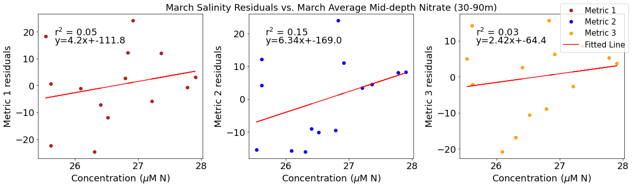
ax4[1].plot(midno3mar,salresid2,'o',color='b',label='Metric 2')
ax4[1].set_xlabel('Concentration ($\mu$M N)')
ax4[1].set_ylabel('Metric 2 residuals')
ax4[1].set_title('March Salinity Residuals vs. March Average Mid-depth Nitrate (30-90m)')
y,r2,m,b=bloomdrivers.reg_r2(midno3mar,salresid2)
ax4[1].plot(midno3mar, y, 'r')
ax4[1].text(0.1, 0.85, '$\mathregular{r^2}$ = %.2f'%r2, transform=ax4[1].transAxes)
ax4[1].text(0.1,0.78,f'y={round(m,2)}x+{round(b,1)}',horizontalalignment='left',verticalalignment='bottom',transform=ax4[1].transAxes)
ax4[2].plot(midno3mar,salresid3,'o',color='orange',label='Metric 3')
ax4[2].set_xlabel('Concentration ($\mu$M N)')
ax4[2].set_ylabel('Metric 3 residuals')
y,r2,m,b=bloomdrivers.reg_r2(midno3mar,salresid3)
ax4[2].plot(midno3mar, y, 'r', label='Fitted Line')
ax4[2].text(0.1, 0.85, '$\mathregular{r^2}$ = %.2f'%r2, transform=ax4[2].transAxes)
ax4[2].text(0.1,0.78,f'y={round(m,2)}x+{round(b,1)}',horizontalalignment='left',verticalalignment='bottom',transform=ax4[2].transAxes)
fig4.legend()
[43]:
<matplotlib.legend.Legend at 0x7f020295adc0>
[44]:
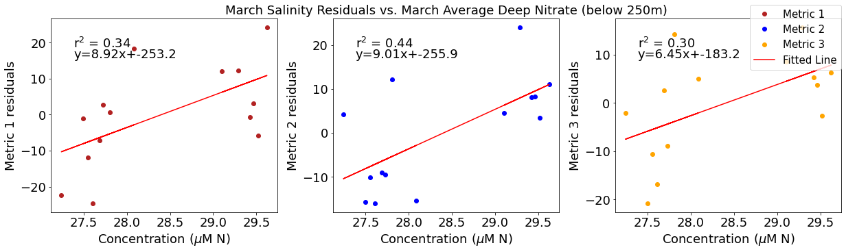
# ---------- Deep NO3 ---------
fig4,ax4=plt.subplots(1,3,figsize=(17,5),constrained_layout=True)
ax4[0].plot(deepno3mar,salresid1,'o',color='firebrick',label='Metric 1')
ax4[0].set_xlabel('Concentration ($\mu$M N)')
ax4[0].set_ylabel('Metric 1 residuals')
y,r2,m,b=bloomdrivers.reg_r2(deepno3mar,salresid1)
ax4[0].plot(deepno3mar, y, 'r')
ax4[0].text(0.1, 0.85, '$\mathregular{r^2}$ = %.2f'%r2, transform=ax4[0].transAxes)
ax4[0].text(0.1,0.78,f'y={round(m,2)}x+{round(b,1)}',horizontalalignment='left',verticalalignment='bottom',transform=ax4[0].transAxes)

ax4[1].plot(deepno3mar,salresid2,'o',color='b',label='Metric 2')
ax4[1].set_xlabel('Concentration ($\mu$M N)')
ax4[1].set_ylabel('Metric 2 residuals')
ax4[1].set_title('March Salinity Residuals vs. March Average Deep Nitrate (below 250m)')
y,r2,m,b=bloomdrivers.reg_r2(deepno3mar,salresid2)
ax4[1].plot(deepno3mar, y, 'r')
ax4[1].text(0.1, 0.85, '$\mathregular{r^2}$ = %.2f'%r2, transform=ax4[1].transAxes)
ax4[1].text(0.1,0.78,f'y={round(m,2)}x+{round(b,1)}',horizontalalignment='left',verticalalignment='bottom',transform=ax4[1].transAxes)

ax4[2].plot(deepno3mar,salresid3,'o',color='orange',label='Metric 3')
ax4[2].set_xlabel('Concentration ($\mu$M N)')
ax4[2].set_ylabel('Metric 3 residuals')
y,r2,m,b=bloomdrivers.reg_r2(deepno3mar,salresid3)
ax4[2].plot(deepno3mar, y, 'r', label='Fitted Line')
ax4[2].text(0.1, 0.85, '$\mathregular{r^2}$ = %.2f'%r2, transform=ax4[2].transAxes)
ax4[2].text(0.1,0.78,f'y={round(m,2)}x+{round(b,1)}',horizontalalignment='left',verticalalignment='bottom',transform=ax4[2].transAxes)
fig4.legend()
[44]:
<matplotlib.legend.Legend at 0x7f02028782b0>
[45]:
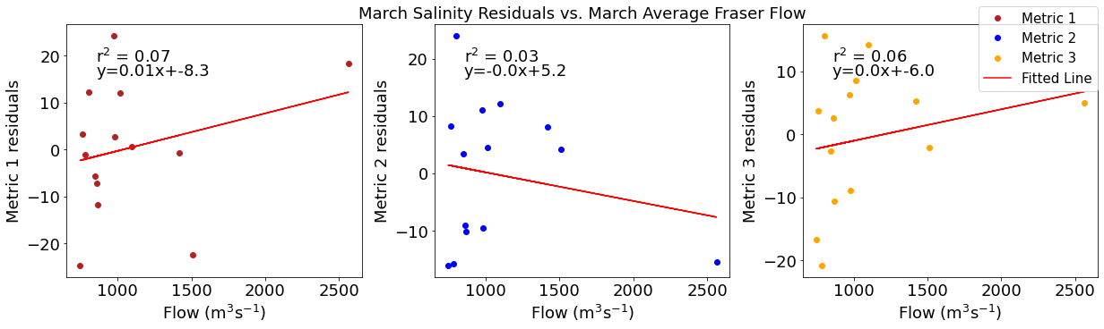
# ---------- Fraser ---------
fig4,ax4=plt.subplots(1,3,figsize=(17,5),constrained_layout=True)
ax4[0].plot(frasermar,salresid1,'o',color='firebrick',label='Metric 1')
ax4[0].set_xlabel('Flow (m$^3$s$^{-1}$)')
ax4[0].set_ylabel('Metric 1 residuals')
y,r2,m,b=bloomdrivers.reg_r2(frasermar,salresid1)
ax4[0].plot(frasermar, y, 'r')
ax4[0].text(0.1, 0.85, '$\mathregular{r^2}$ = %.2f'%r2, transform=ax4[0].transAxes)
ax4[0].text(0.1,0.78,f'y={round(m,2)}x+{round(b,1)}',horizontalalignment='left',verticalalignment='bottom',transform=ax4[0].transAxes)

ax4[1].plot(frasermar,salresid2,'o',color='b',label='Metric 2')
ax4[1].set_xlabel('Flow (m$^3$s$^{-1}$)')
ax4[1].set_ylabel('Metric 2 residuals')
ax4[1].set_title('March Salinity Residuals vs. March Average Fraser Flow')
y,r2,m,b=bloomdrivers.reg_r2(frasermar,salresid2)
ax4[1].plot(frasermar, y, 'r')
ax4[1].text(0.1, 0.85, '$\mathregular{r^2}$ = %.2f'%r2, transform=ax4[1].transAxes)
ax4[1].text(0.1,0.78,f'y={round(m,2)}x+{round(b,1)}',horizontalalignment='left',verticalalignment='bottom',transform=ax4[1].transAxes)

ax4[2].plot(frasermar,salresid3,'o',color='orange',label='Metric 3')
ax4[2].set_xlabel('Flow (m$^3$s$^{-1}$)')
ax4[2].set_ylabel('Metric 3 residuals')
y,r2,m,b=bloomdrivers.reg_r2(frasermar,salresid3)
ax4[2].plot(frasermar, y, 'r', label='Fitted Line')
ax4[2].text(0.1, 0.85, '$\mathregular{r^2}$ = %.2f'%r2, transform=ax4[2].transAxes)
ax4[2].text(0.1,0.78,f'y={round(m,2)}x+{round(b,1)}',horizontalalignment='left',verticalalignment='bottom',transform=ax4[2].transAxes)
fig4.legend()
[45]:
<matplotlib.legend.Legend at 0x7f020270dfa0>
[46]:
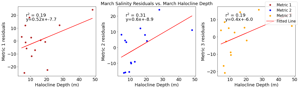
# ---------- Halocline ---------
fig4,ax4=plt.subplots(1,3,figsize=(17,5),constrained_layout=True)
ax4[0].plot(halomar,salresid1,'o',color='firebrick',label='Metric 1')
ax4[0].set_xlabel('Halocline Depth (m)')
ax4[0].set_ylabel('Metric 1 residuals')
y,r2,m,b=bloomdrivers.reg_r2(halomar,salresid1)
ax4[0].plot(halomar, y, 'r')
ax4[0].text(0.1, 0.85, '$\mathregular{r^2}$ = %.2f'%r2, transform=ax4[0].transAxes)
ax4[0].text(0.1,0.78,f'y={round(m,2)}x+{round(b,1)}',horizontalalignment='left',verticalalignment='bottom',transform=ax4[0].transAxes)

ax4[1].plot(halomar,salresid2,'o',color='b',label='Metric 2')
ax4[1].set_xlabel('Halocline Depth (m)')
ax4[1].set_ylabel('Metric 2 residuals')
ax4[1].set_title('March Salinity Residuals vs. March Halocline Depth')
y,r2,m,b=bloomdrivers.reg_r2(halomar,salresid2)
ax4[1].plot(halomar, y, 'r')
ax4[1].text(0.1, 0.85, '$\mathregular{r^2}$ = %.2f'%r2, transform=ax4[1].transAxes)
ax4[1].text(0.1,0.78,f'y={round(m,2)}x+{round(b,1)}',horizontalalignment='left',verticalalignment='bottom',transform=ax4[1].transAxes)

ax4[2].plot(halomar,salresid3,'o',color='orange',label='Metric 3')
ax4[2].set_xlabel('Halocline Depth (m)')
ax4[2].set_ylabel('Metric 3 residuals')
y,r2,m,b=bloomdrivers.reg_r2(halomar,salresid3)
ax4[2].plot(halomar, y, 'r', label='Fitted Line')
ax4[2].text(0.1, 0.85, '$\mathregular{r^2}$ = %.2f'%r2, transform=ax4[2].transAxes)
ax4[2].text(0.1,0.78,f'y={round(m,2)}x+{round(b,1)}',horizontalalignment='left',verticalalignment='bottom',transform=ax4[2].transAxes)
fig4.legend()
[46]:
<matplotlib.legend.Legend at 0x7f0202620520>
Correlation plots of halocline residuals
[47]:
# Wind residual calculations for each metric
haloresid1=list()
y,r2,m,b=bloomdrivers.reg_r2(halomar,yearday1)
for ind,y in enumerate(yearday1):
    x=halomar[ind]
    haloresid1.append(y-(m*x+b))

haloresid2=list()
y,r2,m,b=bloomdrivers.reg_r2(halomar,yearday2)
for ind,y in enumerate(yearday2):
    x=halomar[ind]
    haloresid2.append(y-(m*x+b))

haloresid3=list()
y,r2,m,b=bloomdrivers.reg_r2(halomar,yearday3)
for ind,y in enumerate(yearday3):
    x=halomar[ind]
    haloresid3.append(y-(m*x+b))
[48]:
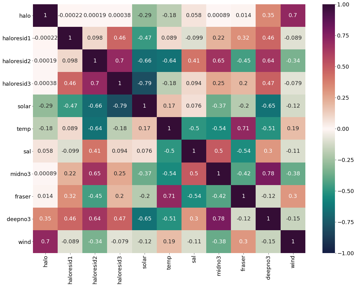
dfhalo=pd.DataFrame({'halo':halomar,'haloresid1':haloresid1,'haloresid2':haloresid2,'haloresid3':haloresid3,'solar':solarmar,
                  'temp':tempmar,'sal':salmar,'midno3':midno3mar,'fraser':frasermar,'deepno3':deepno3mar,'wind':windmar})
[49]:
plt.subplots(figsize=(20,15))
cm1=cmocean.cm.curl
sns.heatmap(dfhalo.corr(), annot = True,cmap=cm1,vmin=-1,vmax=1)
[49]:
<AxesSubplot:>
[50]:
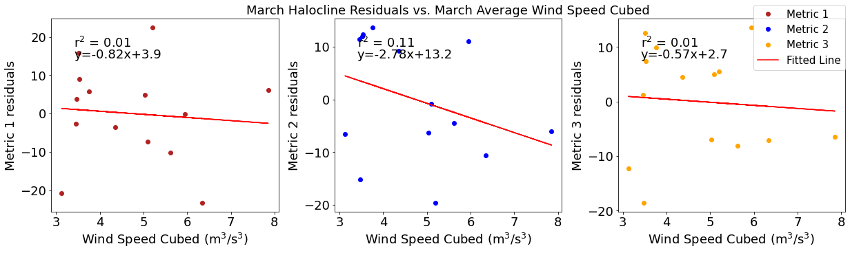
# ---------- wind ---------
fig4,ax4=plt.subplots(1,3,figsize=(17,5),constrained_layout=True)
ax4[0].plot(windmar, haloresid1,'o',color='firebrick',label='Metric 1')
ax4[0].set_xlabel('Wind Speed Cubed ($\mathregular{m^3}$/$\mathregular{s^3}$)')
ax4[0].set_ylabel('Metric 1 residuals')
y,r2,m,b=bloomdrivers.reg_r2(windmar,haloresid1)
ax4[0].plot(windmar, y, 'r')
ax4[0].text(0.1, 0.85, '$\mathregular{r^2}$ = %.2f'%r2, transform=ax4[0].transAxes)
ax4[0].text(0.1,0.78,f'y={round(m,2)}x+{round(b,1)}',horizontalalignment='left',verticalalignment='bottom',transform=ax4[0].transAxes)

ax4[1].plot(windmar,haloresid2,'o',color='b',label='Metric 2')
ax4[1].set_xlabel('Wind Speed Cubed ($\mathregular{m^3}$/$\mathregular{s^3}$)')
ax4[1].set_ylabel('Metric 2 residuals')
ax4[1].set_title('March Halocline Residuals vs. March Average Wind Speed Cubed')
y,r2,m,b=bloomdrivers.reg_r2(windmar,haloresid2)
ax4[1].plot(windmar, y, 'r')
ax4[1].text(0.1, 0.85, '$\mathregular{r^2}$ = %.2f'%r2, transform=ax4[1].transAxes)
ax4[1].text(0.1,0.78,f'y={round(m,2)}x+{round(b,1)}',horizontalalignment='left',verticalalignment='bottom',transform=ax4[1].transAxes)

ax4[2].plot(windmar,haloresid3,'o',color='orange',label='Metric 3')
ax4[2].set_xlabel('Wind Speed Cubed ($\mathregular{m^3}$/$\mathregular{s^3}$)')
ax4[2].set_ylabel('Metric 3 residuals')
y,r2,m,b=bloomdrivers.reg_r2(windmar,haloresid3)
ax4[2].plot(windmar, y, 'r', label='Fitted Line')
ax4[2].text(0.1, 0.85, '$\mathregular{r^2}$ = %.2f'%r2, transform=ax4[2].transAxes)
ax4[2].text(0.1,0.78,f'y={round(m,2)}x+{round(b,1)}',horizontalalignment='left',verticalalignment='bottom',transform=ax4[2].transAxes)
fig4.legend()
[50]:
<matplotlib.legend.Legend at 0x7f02023b2880>
[51]:
# ---------- Solar ---------
fig4,ax4=plt.subplots(1,3,figsize=(17,5),constrained_layout=True)
ax4[0].plot(solarmar,haloresid1,'o',color='firebrick',label='Metric 1')
ax4[0].set_xlabel('Solar Irradiance (W/$\mathregular{m^2}$)')
ax4[0].set_ylabel('Metric 1 residuals')
y,r2,m,b=bloomdrivers.reg_r2(solarmar,haloresid1)
ax4[0].plot(solarmar, y, 'r')
ax4[0].text(0.1, 0.85, '$\mathregular{r^2}$ = %.2f'%r2, transform=ax4[0].transAxes)
ax4[0].text(0.1,0.78,f'y={round(m,2)}x+{round(b,1)}',horizontalalignment='left',verticalalignment='bottom',transform=ax4[0].transAxes)

ax4[1].plot(solarmar,haloresid2,'o',color='b',label='Metric 2')
ax4[1].set_xlabel('Solar Irradiance (W/$\mathregular{m^2}$)')
ax4[1].set_ylabel('Metric 2 residuals')
ax4[1].set_title('March Halocline Residuals vs. March Average Solar Radiation')
y,r2,m,b=bloomdrivers.reg_r2(solarmar,haloresid2)
ax4[1].plot(solarmar, y, 'r')
ax4[1].text(0.1, 0.85, '$\mathregular{r^2}$ = %.2f'%r2, transform=ax4[1].transAxes)
ax4[1].text(0.1,0.78,f'y={round(m,2)}x+{round(b,1)}',horizontalalignment='left',verticalalignment='bottom',transform=ax4[1].transAxes)

ax4[2].plot(solarmar,haloresid3,'o',color='orange',label='Metric 3')
ax4[2].set_xlabel('Solar Irradiance (W/$\mathregular{m^2}$)')
ax4[2].set_ylabel('Metric 3 residuals')
y,r2,m,b=bloomdrivers.reg_r2(solarmar,haloresid3)
ax4[2].plot(solarmar, y, 'r', label='Fitted Line')
ax4[2].text(0.1, 0.85, '$\mathregular{r^2}$ = %.2f'%r2, transform=ax4[2].transAxes)
ax4[2].text(0.1,0.78,f'y={round(m,2)}x+{round(b,1)}',horizontalalignment='left',verticalalignment='bottom',transform=ax4[2].transAxes)
fig4.legend()
[51]:
<matplotlib.legend.Legend at 0x7f02022bd970>
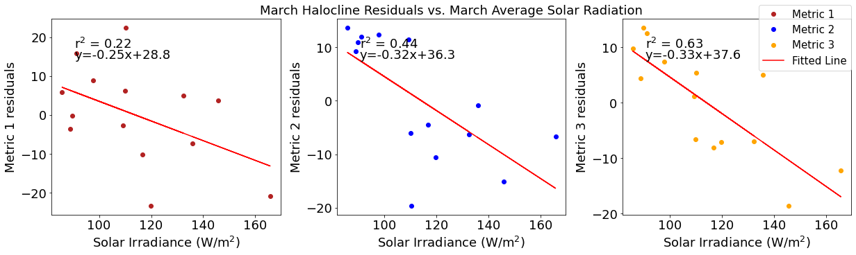
[52]:
# ---------- Temperature ---------
fig4,ax4=plt.subplots(1,3,figsize=(17,5),constrained_layout=True)
ax4[0].plot(tempmar,haloresid1,'o',color='firebrick',label='Metric 1')
ax4[0].set_xlabel('Surface Temperature ($^\circ$C)')
ax4[0].set_ylabel('Metric 1 residuals')
y,r2,m,b=bloomdrivers.reg_r2(tempmar,haloresid1)
ax4[0].plot(tempmar, y, 'r')
ax4[0].text(0.1, 0.85, '$\mathregular{r^2}$ = %.2f'%r2, transform=ax4[0].transAxes)
ax4[0].text(0.1,0.78,f'y={round(m,2)}x+{round(b,1)}',horizontalalignment='left',verticalalignment='bottom',transform=ax4[0].transAxes)

ax4[1].plot(tempmar,haloresid2,'o',color='b',label='Metric 2')
ax4[1].set_xlabel('Surface Temperature ($^\circ$C)')
ax4[1].set_ylabel('Metric 2 residuals')
ax4[1].set_title('March Halocline Residuals vs. March Average Surface Temperature')
y,r2,m,b=bloomdrivers.reg_r2(tempmar,haloresid2)
ax4[1].plot(tempmar, y, 'r')
ax4[1].text(0.1, 0.85, '$\mathregular{r^2}$ = %.2f'%r2, transform=ax4[1].transAxes)
ax4[1].text(0.1,0.78,f'y={round(m,2)}x+{round(b,1)}',horizontalalignment='left',verticalalignment='bottom',transform=ax4[1].transAxes)

ax4[2].plot(tempmar,haloresid3,'o',color='orange',label='Metric 3')
ax4[2].set_xlabel('Surface Temperature ($^\circ$C)')
ax4[2].set_ylabel('Metric 3 residuals')
y,r2,m,b=bloomdrivers.reg_r2(tempmar,haloresid3)
ax4[2].plot(tempmar, y, 'r', label='Fitted Line')
ax4[2].text(0.1, 0.85, '$\mathregular{r^2}$ = %.2f'%r2, transform=ax4[2].transAxes)
ax4[2].text(0.1,0.78,f'y={round(m,2)}x+{round(b,1)}',horizontalalignment='left',verticalalignment='bottom',transform=ax4[2].transAxes)
fig4.legend()
[52]:
<matplotlib.legend.Legend at 0x7f0202158dc0>
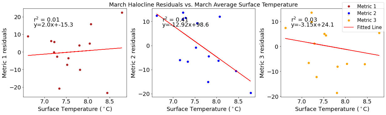
[53]:
# ---------- Deep NO3 ---------
fig4,ax4=plt.subplots(1,3,figsize=(17,5),constrained_layout=True)
ax4[0].plot(midno3mar,haloresid1,'o',color='firebrick',label='Metric 1')
ax4[0].set_xlabel('Concentration ($\mu$M N)')
ax4[0].set_ylabel('Metric 1 residuals')
y,r2,m,b=bloomdrivers.reg_r2(midno3mar,haloresid1)
ax4[0].plot(midno3mar, y, 'r')
ax4[0].text(0.1, 0.85, '$\mathregular{r^2}$ = %.2f'%r2, transform=ax4[0].transAxes)
ax4[0].text(0.1,0.78,f'y={round(m,2)}x+{round(b,1)}',horizontalalignment='left',verticalalignment='bottom',transform=ax4[0].transAxes)

ax4[1].plot(midno3mar,haloresid2,'o',color='b',label='Metric 2')
ax4[1].set_xlabel('Concentration ($\mu$M N)')
ax4[1].set_ylabel('Metric 2 residuals')
ax4[1].set_title('March Halocline Residuals vs. March Average Mid-depth Nitrate (30-90m)')
y,r2,m,b=bloomdrivers.reg_r2(midno3mar,haloresid2)
ax4[1].plot(midno3mar, y, 'r')
ax4[1].text(0.1, 0.85, '$\mathregular{r^2}$ = %.2f'%r2, transform=ax4[1].transAxes)
ax4[1].text(0.1,0.78,f'y={round(m,2)}x+{round(b,1)}',horizontalalignment='left',verticalalignment='bottom',transform=ax4[1].transAxes)

ax4[2].plot(midno3mar,haloresid3,'o',color='orange',label='Metric 3')
ax4[2].set_xlabel('Concentration ($\mu$M N)')
ax4[2].set_ylabel('Metric 3 residuals')
y,r2,m,b=bloomdrivers.reg_r2(midno3mar,haloresid3)
ax4[2].plot(midno3mar, y, 'r', label='Fitted Line')
ax4[2].text(0.1, 0.85, '$\mathregular{r^2}$ = %.2f'%r2, transform=ax4[2].transAxes)
ax4[2].text(0.1,0.78,f'y={round(m,2)}x+{round(b,1)}',horizontalalignment='left',verticalalignment='bottom',transform=ax4[2].transAxes)
fig4.legend()
[53]:
<matplotlib.legend.Legend at 0x7f02020706a0>
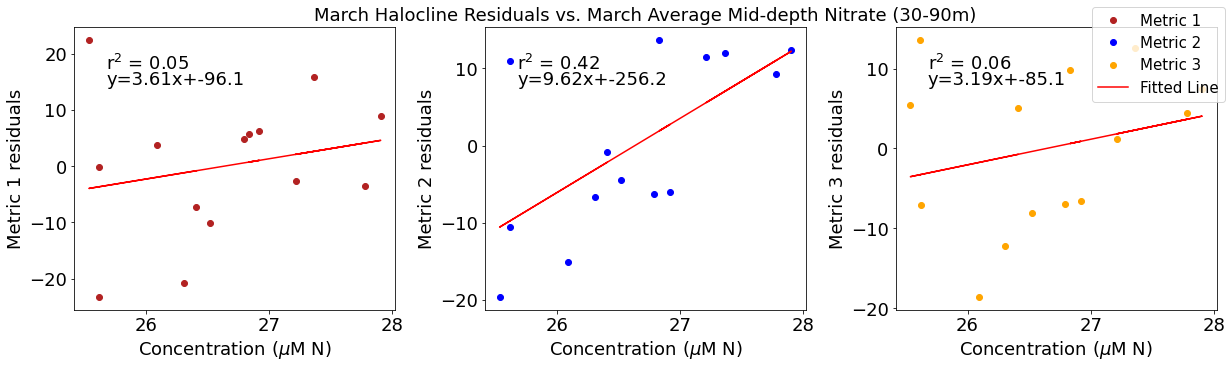
[54]:
# ---------- Deep NO3 ---------
fig4,ax4=plt.subplots(1,3,figsize=(17,5),constrained_layout=True)
ax4[0].plot(deepno3mar,haloresid1,'o',color='firebrick',label='Metric 1')
ax4[0].set_xlabel('Concentration ($\mu$M N)')
ax4[0].set_ylabel('Metric 1 residuals')
y,r2,m,b=bloomdrivers.reg_r2(deepno3mar,haloresid1)
ax4[0].plot(deepno3mar, y, 'r')
ax4[0].text(0.1, 0.85, '$\mathregular{r^2}$ = %.2f'%r2, transform=ax4[0].transAxes)
ax4[0].text(0.1,0.78,f'y={round(m,2)}x+{round(b,1)}',horizontalalignment='left',verticalalignment='bottom',transform=ax4[0].transAxes)

ax4[1].plot(deepno3mar,haloresid2,'o',color='b',label='Metric 2')
ax4[1].set_xlabel('Concentration ($\mu$M N)')
ax4[1].set_ylabel('Metric 2 residuals')
ax4[1].set_title('March Halocline Residuals vs. March Average Deep Nitrate (below 250m)')
y,r2,m,b=bloomdrivers.reg_r2(deepno3mar,haloresid2)
ax4[1].plot(deepno3mar, y, 'r')
ax4[1].text(0.1, 0.85, '$\mathregular{r^2}$ = %.2f'%r2, transform=ax4[1].transAxes)
ax4[1].text(0.1,0.78,f'y={round(m,2)}x+{round(b,1)}',horizontalalignment='left',verticalalignment='bottom',transform=ax4[1].transAxes)

ax4[2].plot(deepno3mar,haloresid3,'o',color='orange',label='Metric 3')
ax4[2].set_xlabel('Concentration ($\mu$M N)')
ax4[2].set_ylabel('Metric 3 residuals')
y,r2,m,b=bloomdrivers.reg_r2(deepno3mar,haloresid3)
ax4[2].plot(deepno3mar, y, 'r', label='Fitted Line')
ax4[2].text(0.1, 0.85, '$\mathregular{r^2}$ = %.2f'%r2, transform=ax4[2].transAxes)
ax4[2].text(0.1,0.78,f'y={round(m,2)}x+{round(b,1)}',horizontalalignment='left',verticalalignment='bottom',transform=ax4[2].transAxes)
fig4.legend()
[54]:
<matplotlib.legend.Legend at 0x7f020339f100>
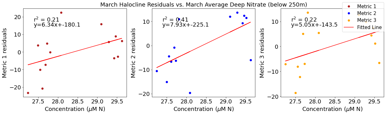
[55]:
# ---------- Fraser ---------
fig4,ax4=plt.subplots(1,3,figsize=(17,5),constrained_layout=True)
ax4[0].plot(frasermar,haloresid1,'o',color='firebrick',label='Metric 1')
ax4[0].set_xlabel('Flow (m$^3$s$^{-1}$)')
ax4[0].set_ylabel('Metric 1 residuals')
y,r2,m,b=bloomdrivers.reg_r2(frasermar,haloresid1)
ax4[0].plot(frasermar, y, 'r')
ax4[0].text(0.1, 0.85, '$\mathregular{r^2}$ = %.2f'%r2, transform=ax4[0].transAxes)
ax4[0].text(0.1,0.78,f'y={round(m,2)}x+{round(b,1)}',horizontalalignment='left',verticalalignment='bottom',transform=ax4[0].transAxes)

ax4[1].plot(frasermar,haloresid2,'o',color='b',label='Metric 2')
ax4[1].set_xlabel('Flow (m$^3$s$^{-1}$)')
ax4[1].set_ylabel('Metric 2 residuals')
ax4[1].set_title('March Halocline Residuals vs. March Average Fraser Flow')
y,r2,m,b=bloomdrivers.reg_r2(frasermar,haloresid2)
ax4[1].plot(frasermar, y, 'r')
ax4[1].text(0.1, 0.85, '$\mathregular{r^2}$ = %.2f'%r2, transform=ax4[1].transAxes)
ax4[1].text(0.1,0.78,f'y={round(m,2)}x+{round(b,1)}',horizontalalignment='left',verticalalignment='bottom',transform=ax4[1].transAxes)

ax4[2].plot(frasermar,haloresid3,'o',color='orange',label='Metric 3')
ax4[2].set_xlabel('Flow (m$^3$s$^{-1}$)')
ax4[2].set_ylabel('Metric 3 residuals')
y,r2,m,b=bloomdrivers.reg_r2(frasermar,haloresid2)
ax4[2].plot(frasermar, y, 'r', label='Fitted Line')
ax4[2].text(0.1, 0.85, '$\mathregular{r^2}$ = %.2f'%r2, transform=ax4[2].transAxes)
ax4[2].text(0.1,0.78,f'y={round(m,2)}x+{round(b,1)}',horizontalalignment='left',verticalalignment='bottom',transform=ax4[2].transAxes)
fig4.legend()
[55]:
<matplotlib.legend.Legend at 0x7f0201e887f0>
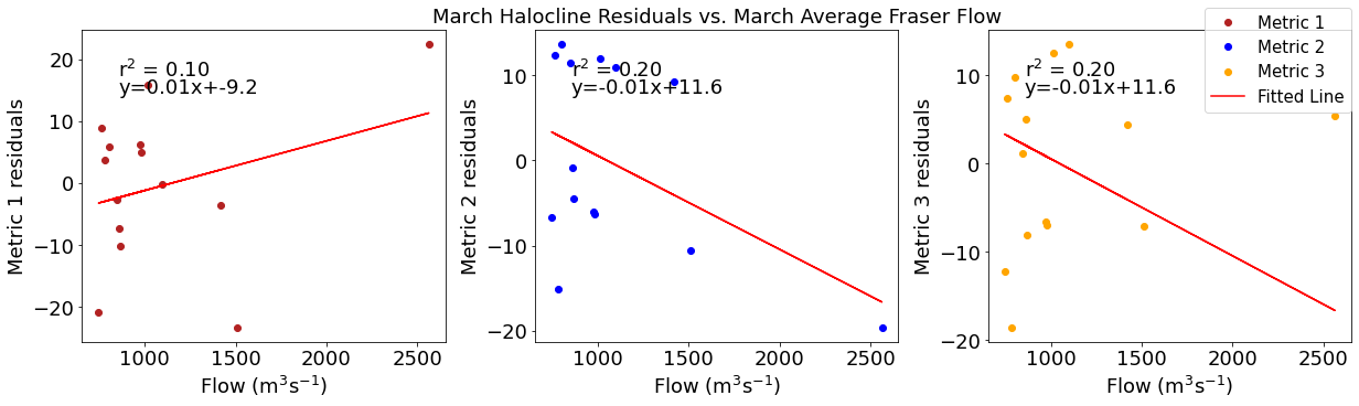
[56]:
# ---------- Salinity ---------
fig4,ax4=plt.subplots(1,3,figsize=(17,5),constrained_layout=True)
ax4[0].plot(salmar,haloresid1,'o',color='firebrick',label='Metric 1')
ax4[0].set_xlabel('Salinity (g/kg)')
ax4[0].set_ylabel('Metric 1 residuals')
y,r2,m,b=bloomdrivers.reg_r2(salmar,haloresid1)
ax4[0].plot(salmar, y, 'r')
ax4[0].text(0.1, 0.85, '$\mathregular{r^2}$ = %.2f'%r2, transform=ax4[0].transAxes)
ax4[0].text(0.1,0.78,f'y={round(m,2)}x+{round(b,1)}',horizontalalignment='left',verticalalignment='bottom',transform=ax4[0].transAxes)

ax4[1].plot(salmar,haloresid2,'o',color='b',label='Metric 2')
ax4[1].set_xlabel('Salinity (g/kg)')
ax4[1].set_ylabel('Metric 2 residuals')
ax4[1].set_title('March Halocline Residuals vs. March Average Absolute Surface Salinity')
y,r2,m,b=bloomdrivers.reg_r2(salmar,haloresid2)
ax4[1].plot(salmar, y, 'r')
ax4[1].text(0.1, 0.85, '$\mathregular{r^2}$ = %.2f'%r2, transform=ax4[1].transAxes)
ax4[1].text(0.1,0.78,f'y={round(m,2)}x+{round(b,1)}',horizontalalignment='left',verticalalignment='bottom',transform=ax4[1].transAxes)

ax4[2].plot(salmar,haloresid3,'o',color='orange',label='Metric 3')
ax4[2].set_xlabel('Salinity (g/kg)')
ax4[2].set_ylabel('Metric 3 residuals')
y,r2,m,b=bloomdrivers.reg_r2(salmar,haloresid3)
ax4[2].plot(salmar, y, 'r', label='Fitted Line')
ax4[2].text(0.1, 0.85, '$\mathregular{r^2}$ = %.2f'%r2, transform=ax4[2].transAxes)
ax4[2].text(0.1,0.78,f'y={round(m,2)}x+{round(b,1)}',horizontalalignment='left',verticalalignment='bottom',transform=ax4[2].transAxes)
fig4.legend()
[56]:
<matplotlib.legend.Legend at 0x7f0201db1220>
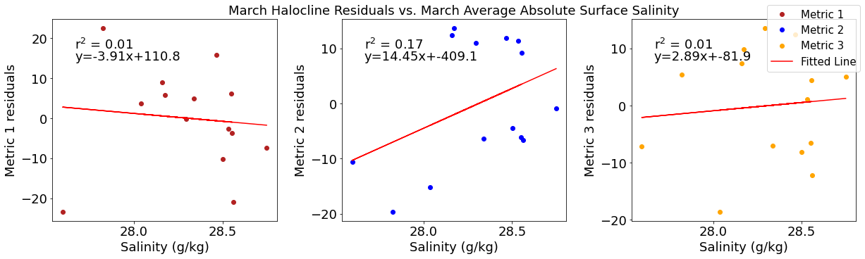
Multiple linear regression
Correlation with winds (least to greatest) * Salinity, solar, deep no3, temp, fraser, midno3, halocline
Correlation with solar * Salinity, wind, temp, fraser, halocline, midno3, deep no3
Correlation with temperature * Solar, halocline wind, salinity, deep no3, midno3, fraser
Correlation with midno3 * Halocline, solar, wind, fraser, sal, temp, depp no3
Correlation with deep no3 * Fraser wind, sal, halocline, temp, solar, mid no3
Correlation with salinity * Halocline, solar, wind, deepno3, temp/midno3, fraser
Correlation with fraser * Halocline, deepno3, solar, wind, midno3, sal, temp
Correlation with halocline * Midno3, fraser, sal, temp, solar, deepno3, wind
[57]:
# make a table
variables=list()
rsquared=list()
adjusted_r2=list()
MLR with january deepno3+salinity+temp, and bloom date:
[58]:
A=np.vstack((deepno3jan,saljan,tempjan,np.ones(np.shape(tempjan)))).T
b=yearday2
m=np.linalg.lstsq(A,b,rcond=None)[0]
model, resid = np.linalg.lstsq(A, b,rcond=None)[:2]
r2 = 1 - resid / (len(b) * np.var(b))
p=3 # number of parameters
ar2= 1-(len(b)-1)/(len(b)-p)*(1-r2)
print('Coefficients and intercept:')
print(m)
print('r2 value:')
print(r2)
print('adjusted r2 value:')
print(ar2)
variables.append('deepno3jan,saljan,tempjan')
rsquared.append(r2)
adjusted_r2.append(ar2)
Coefficients and intercept:
[   9.75563259   10.49966658   -7.88209314 -415.19733104]
r2 value:
[0.65180813]
adjusted r2 value:
[0.58850052]
MLR with feb deepno3+salinity+solar and bloom date:
[59]:
A=np.vstack((deepno3feb,salfeb,solarfeb,np.ones(np.shape(salfeb)))).T
b=yearday2
m=np.linalg.lstsq(A,b,rcond=None)[0]
model, resid = np.linalg.lstsq(A, b,rcond=None)[:2]
r2 = 1 - resid / (len(b) * np.var(b))
p=3 # number of parameters
ar2= 1-(len(b)-1)/(len(b)-p)*(1-r2)
print('Coefficients and intercept:')
print(m)
print('r2 value:')
print(r2)
print('adjusted r2 value:')
print(ar2)
variables.append('deepno3feb,salfeb,solarfeb')
rsquared.append(r2)
adjusted_r2.append(ar2)
Coefficients and intercept:
[   9.33069212    1.86124695   -0.24535405 -199.36963347]
r2 value:
[0.54967335]
adjusted r2 value:
[0.46779578]
MLR with feb midno3+solar+temp and bloom date:
[60]:
A=np.vstack((midno3feb,solarfeb,tempfeb,np.ones(np.shape(solarfeb)))).T
b=yearday2
m=np.linalg.lstsq(A,b,rcond=None)[0]
model, resid = np.linalg.lstsq(A, b,rcond=None)[:2]
r2 = 1 - resid / (len(b) * np.var(b))
p=3 # number of parameters
ar2= 1-(len(b)-1)/(len(b)-p)*(1-r2)
print('Coefficients and intercept:')
print(m)
print('r2 value:')
print(r2)
print('adjusted r2 value:')
print(ar2)
variables.append('midno3feb,solarfeb,tempfeb')
rsquared.append(r2)
adjusted_r2.append(ar2)
Coefficients and intercept:
[ -2.98681065  -0.97603155 -12.55783965 331.33244477]
r2 value:
[0.6342635]
adjusted r2 value:
[0.56776595]
MLR with march solar+deepno3+halocline, and bloom date:
[61]:
A=np.vstack((solarmar,deepno3mar,halomar,np.ones(np.shape(solarmar)))).T
b=yearday2
m=np.linalg.lstsq(A,b,rcond=None)[0]
model, resid = np.linalg.lstsq(A, b,rcond=None)[:2]
r2 = 1 - resid / (len(b) * np.var(b))
p=3 # number of parameters
ar2= 1-(len(b)-1)/(len(b)-p)*(1-r2)
print('Coefficients and intercept:')
print(m)
print('r2 value:')
print(r2)
print('adjusted r2 value:')
print(ar2)
variables.append('solarmar,deepno3mar,halomar')
rsquared.append(r2)
adjusted_r2.append(ar2)
Coefficients and intercept:
[ -0.22002608   5.4790777    0.34732453 -35.52738868]
r2 value:
[0.71021129]
adjusted r2 value:
[0.65752243]
MLR with solar+deepno3, and bloom date:
[62]:
A=np.vstack((solarmar,deepno3mar,np.ones(np.shape(solarmar)))).T
b=yearday2
m=np.linalg.lstsq(A,b,rcond=None)[0]
model, resid = np.linalg.lstsq(A, b,rcond=None)[:2]
r2 = 1 - resid / (len(b) * np.var(b))
p=2 # number of parameters
ar2= 1-(len(b)-1)/(len(b)-p)*(1-r2)
print('Coefficients and intercept:')
print(m)
print('r2 value:')
print(r2)
print('adjusted r2 value:')
print(ar2)
variables.append('solarmar,deepno3mar')
rsquared.append(r2)
adjusted_r2.append(ar2)
Coefficients and intercept:
[ -0.23892842   6.68378623 -62.4653773 ]
r2 value:
[0.63176615]
adjusted r2 value:
[0.60108]
MLR with solar+halocline, and bloom date:
[63]:
A=np.vstack((solarmar,halomar,np.ones(np.shape(solarmar)))).T
b=yearday2
m=np.linalg.lstsq(A,b,rcond=None)[0]
model, resid = np.linalg.lstsq(A, b,rcond=None)[:2]
r2 = 1 - resid / (len(b) * np.var(b))
p=2 # number of parameters
ar2= 1-(len(b)-1)/(len(b)-p)*(1-r2)
print('Coefficients and intercept:')
print(m)
print('r2 value:')
print(r2)
print('adjusted r2 value:')
print(ar2)
variables.append('solarmar,halomar')
rsquared.append(r2)
adjusted_r2.append(ar2)
Coefficients and intercept:
[ -0.34668156   0.42269898 133.44362134]
r2 value:
[0.63278647]
adjusted r2 value:
[0.60218534]
MLR with deepno3+halocline, and bloom date:
[64]:
A=np.vstack((deepno3mar,halomar,np.ones(np.shape(halomar)))).T
b=yearday2
m=np.linalg.lstsq(A,b,rcond=None)[0]
model, resid = np.linalg.lstsq(A, b,rcond=None)[:2]
r2 = 1 - resid / (len(b) * np.var(b))
p=2 # number of parameters
ar2= 1-(len(b)-1)/(len(b)-p)*(1-r2)
print('Coefficients and intercept:')
print(m)
print('r2 value:')
print(r2)
print('adjusted r2 value:')
print(ar2)
variables.append('deepno3mar,halomar')
rsquared.append(r2)
adjusted_r2.append(ar2)
Coefficients and intercept:
[   9.00163186    0.38021664 -161.19135546]
r2 value:
[0.62373828]
adjusted r2 value:
[0.59238313]
MLR with feb midno3+march solar, and bloom date:
[65]:
A=np.vstack((midno3feb,solarmar,np.ones(np.shape(solarmar)))).T
b=yearday2
m=np.linalg.lstsq(A,b,rcond=None)[0]
model, resid = np.linalg.lstsq(A, b,rcond=None)[:2]
r2 = 1 - resid / (len(b) * np.var(b))
p=2 # number of parameters
ar2= 1-(len(b)-1)/(len(b)-p)*(1-r2)
print('Coefficients and intercept:')
print(m)
print('r2 value:')
print(r2)
print('adjusted r2 value:')
print(ar2)
variables.append('midno3feb,solarmar')
rsquared.append(r2)
adjusted_r2.append(ar2)
Coefficients and intercept:
[ 5.07335825 -0.32640808 -0.12420413]
r2 value:
[0.57754578]
adjusted r2 value:
[0.54234126]
MLR with feb midno3+march solar+march temp, and bloom date:
[66]:
A=np.vstack((midno3feb,solarmar,tempmar,np.ones(np.shape(solarmar)))).T
b=yearday2
m=np.linalg.lstsq(A,b,rcond=None)[0]
model, resid = np.linalg.lstsq(A, b,rcond=None)[:2]
r2 = 1 - resid / (len(b) * np.var(b))
p=3 # number of parameters
ar2= 1-(len(b)-1)/(len(b)-p)*(1-r2)
print('Coefficients and intercept:')
print(m)
print('r2 value:')
print(r2)
print('adjusted r2 value:')
print(ar2)
variables.append('midno3feb,solarmar,tempmar')
rsquared.append(r2)
adjusted_r2.append(ar2)
Coefficients and intercept:
[  0.59306092  -0.3474031  -12.45501673 218.75674844]
r2 value:
[0.7900923]
adjusted r2 value:
[0.75192726]
MLR with feb midno3 and bloom date:
[67]:
A=np.vstack((midno3feb,np.ones(np.shape(midno3feb)))).T
b=yearday2
m=np.linalg.lstsq(A,b,rcond=None)[0]
model, resid = np.linalg.lstsq(A, b,rcond=None)[:2]
r2 = 1 - resid / (len(b) * np.var(b))
p=1 # number of parameters
ar2= 1-(len(b)-1)/(len(b)-p)*(1-r2)
print('Coefficients and intercept:')
print(m)
print('r2 value:')
print(r2)
print('adjusted r2 value:')
print(ar2)
variables.append('midno3feb')
rsquared.append(r2)
adjusted_r2.append(ar2)
Coefficients and intercept:
[   9.80665078 -165.6753908 ]
r2 value:
[0.32345092]
adjusted r2 value:
[0.32345092]
MLR with march solar and bloom date:
[68]:
A=np.vstack((solarmar,np.ones(np.shape(solarmar)))).T
b=yearday2
m=np.linalg.lstsq(A,b,rcond=None)[0]
model, resid = np.linalg.lstsq(A, b,rcond=None)[:2]
r2 = 1 - resid / (len(b) * np.var(b))
p=1 # number of parameters
ar2= 1-(len(b)-1)/(len(b)-p)*(1-r2)
print('Coefficients and intercept:')
print(m)
print('r2 value:')
print(r2)
print('adjusted r2 value:')
print(ar2)
variables.append('solarmar')
rsquared.append(r2)
adjusted_r2.append(ar2)
Coefficients and intercept:
[ -0.40642865 146.49757367]
r2 value:
[0.51077771]
adjusted r2 value:
[0.51077771]
MLR with march temp and bloom date:
[69]:
A=np.vstack((tempmar,np.ones(np.shape(tempmar)))).T
b=yearday2
m=np.linalg.lstsq(A,b,rcond=None)[0]
model, resid = np.linalg.lstsq(A, b,rcond=None)[:2]
r2 = 1 - resid / (len(b) * np.var(b))
p=1 # number of parameters
ar2= 1-(len(b)-1)/(len(b)-p)*(1-r2)
print('Coefficients and intercept:')
print(m)
print('r2 value:')
print(r2)
print('adjusted r2 value:')
print(ar2)
variables.append('tempmar')
rsquared.append(r2)
adjusted_r2.append(ar2)
Coefficients and intercept:
[-15.27717805 216.6865827 ]
r2 value:
[0.40959944]
adjusted r2 value:
[0.40959944]
MLR with march solar+temp+densdiff30 and bloom date:
[70]:
A=np.vstack((densdiff30mar,solarmar,tempmar,np.ones(np.shape(solarmar)))).T
b=yearday2
m=np.linalg.lstsq(A,b,rcond=None)[0]
model, resid = np.linalg.lstsq(A, b,rcond=None)[:2]
r2 = 1 - resid / (len(b) * np.var(b))
p=3 # number of parameters
ar2= 1-(len(b)-1)/(len(b)-p)*(1-r2)
print('Coefficients and intercept:')
print(m)
print('r2 value:')
print(r2)
print('adjusted r2 value:')
print(ar2)
variables.append('solarmar,tempmar,densdiff30mar')
rsquared.append(r2)
adjusted_r2.append(ar2)
Coefficients and intercept:
[-20.58583808  -0.29989851 -11.08444723 235.13728731]
r2 value:
[0.90631533]
adjusted r2 value:
[0.88928175]
MLR with march solar+temp and bloom date:
[71]:
A=np.vstack((solarmar,tempmar,np.ones(np.shape(solarmar)))).T
b=yearday2
m=np.linalg.lstsq(A,b,rcond=None)[0]
model, resid = np.linalg.lstsq(A, b,rcond=None)[:2]
r2 = 1 - resid / (len(b) * np.var(b))
p=2 # number of parameters
ar2= 1-(len(b)-1)/(len(b)-p)*(1-r2)
print('Coefficients and intercept:')
print(m)
print('r2 value:')
print(r2)
print('adjusted r2 value:')
print(ar2)
variables.append('solarmar,tempmar')
rsquared.append(r2)
adjusted_r2.append(ar2)
Coefficients and intercept:
[ -0.35546345 -12.77943888 238.22502757]
r2 value:
[0.78935945]
adjusted r2 value:
[0.77180608]
MLR with march solar+halo and bloom date:
[72]:
A=np.vstack((solarmar,halomar,np.ones(np.shape(solarmar)))).T
b=yearday2
m=np.linalg.lstsq(A,b,rcond=None)[0]
model, resid = np.linalg.lstsq(A, b,rcond=None)[:2]
r2 = 1 - resid / (len(b) * np.var(b))
p=2 # number of parameters
ar2= 1-(len(b)-1)/(len(b)-p)*(1-r2)
print('Coefficients and intercept:')
print(m)
print('r2 value:')
print(r2)
print('adjusted r2 value:')
print(ar2)
variables.append('solarmar,halomar')
rsquared.append(r2)
adjusted_r2.append(ar2)
Coefficients and intercept:
[ -0.34668156   0.42269898 133.44362134]
r2 value:
[0.63278647]
adjusted r2 value:
[0.60218534]
MLR with march solar+densdiff30 and bloom date:
[73]:
A=np.vstack((solarmar,densdiff30mar,np.ones(np.shape(solarmar)))).T
b=yearday2
m=np.linalg.lstsq(A,b,rcond=None)[0]
model, resid = np.linalg.lstsq(A, b,rcond=None)[:2]
r2 = 1 - resid / (len(b) * np.var(b))
p=2 # number of parameters
ar2= 1-(len(b)-1)/(len(b)-p)*(1-r2)
print('Coefficients and intercept:')
print(m)
print('r2 value:')
print(r2)
print('adjusted r2 value:')
print(ar2)
variables.append('solarmar,densdiff30mar')
rsquared.append(r2)
adjusted_r2.append(ar2)
Coefficients and intercept:
[ -0.32771236 -25.99998483 157.96370557]
r2 value:
[0.70516072]
adjusted r2 value:
[0.68059078]
MLR with march solar+temp+halocline and bloom date:
[74]:
A=np.vstack((solarmar,tempmar,halomar,np.ones(np.shape(solarmar)))).T
b=yearday2
m=np.linalg.lstsq(A,b,rcond=None)[0]
model, resid = np.linalg.lstsq(A, b,rcond=None)[:2]
r2 = 1 - resid / (len(b) * np.var(b))
p=3 # number of parameters
ar2= 1-(len(b)-1)/(len(b)-p)*(1-r2)
print('Coefficients and intercept:')
print(m)
print('r2 value:')
print(r2)
print('adjusted r2 value:')
print(ar2)
variables.append('solarmar,tempmar,halomar')
rsquared.append(r2)
adjusted_r2.append(ar2)
Coefficients and intercept:
[ -0.31144302 -11.81502883   0.33864654 220.84453338]
r2 value:
[0.86608374]
adjusted r2 value:
[0.84173533]
[ ]:
[75]:
mlr_df=pd.DataFrame({'Environmental Drivers':variables,'R-squared':rsquared,'Adjusted R-squared':adjusted_r2})
mlr_df.sort_values(by=['Adjusted R-squared'],ascending=False,inplace=True)
mlr_df
[75]:
| Environmental Drivers | R-squared | Adjusted R-squared | |
|---|---|---|---|
| 12 | solarmar,tempmar,densdiff30mar | [0.9063153278500765] | [0.889281751095545] |
| 16 | solarmar,tempmar,halomar | [0.8660837442574524] | [0.8417353341224437] |
| 13 | solarmar,tempmar | [0.78935945447974] | [0.771806075686385] |
| 8 | midno3feb,solarmar,tempmar | [0.7900923003497292] | [0.7519272640496799] |
| 15 | solarmar,densdiff30mar | [0.7051607193847842] | [0.6805907793335162] |
| 3 | solarmar,deepno3mar,halomar | [0.7102112879130422] | [0.657522431169959] |
| 5 | solarmar,halomar | [0.6327864680166315] | [0.6021853403513509] |
| 14 | solarmar,halomar | [0.6327864680166315] | [0.6021853403513509] |
| 4 | solarmar,deepno3mar | [0.6317661500743295] | [0.6010799959138569] |
| 6 | deepno3mar,halomar | [0.6237382755092498] | [0.5923831318016872] |
| 0 | deepno3jan,saljan,tempjan | [0.6518081319696515] | [0.5885005196004972] |
| 2 | midno3feb,solarfeb,tempfeb | [0.6342634950209916] | [0.5677659486611718] |
| 7 | midno3feb,solarmar | [0.5775457809316078] | [0.5423412626759085] |
| 10 | solarmar | [0.5107777148770687] | [0.5107777148770687] |
| 1 | deepno3feb,salfeb,solarfeb | [0.549673352131961] | [0.46779577979231757] |
| 11 | tempmar | [0.4095994360778237] | [0.4095994360778237] |
| 9 | midno3feb | [0.32345092304089984] | [0.32345092304089984] |
Table for report
[92]:
# make a table
variables=list()
rsquared=list()
adjusted_r2=list()
MLR with density30, and bloom date:
[93]:
A=np.vstack((densdiff30mar,np.ones(np.shape(windmar)))).T
b=yearday2
m=np.linalg.lstsq(A,b,rcond=None)[0]
model, resid = np.linalg.lstsq(A, b,rcond=None)[:2]
r2 = 1 - resid / (len(b) * np.var(b))
p=1 # number of parameters
ar2= 1-(len(b)-1)/(len(b)-p)*(1-r2)
print('Coefficients and intercept:')
print(m)
print('r2 value:')
print(r2)
print('adjusted r2 value:')
print(ar2)
variables.append('Density Difference 30m')
rsquared.append(np.round(r2,2))
adjusted_r2.append(np.round(ar2,2))
Coefficients and intercept:
[-35.71198635 128.17108402]
r2 value:
[0.40287183]
adjusted r2 value:
[0.40287183]
MLR with solar, and bloom date:
[94]:
A=np.vstack((solarmar,np.ones(np.shape(windmar)))).T
b=yearday2
m=np.linalg.lstsq(A,b,rcond=None)[0]
model, resid = np.linalg.lstsq(A, b,rcond=None)[:2]
r2 = 1 - resid / (len(b) * np.var(b))
p=1 # number of parameters
ar2= 1-(len(b)-1)/(len(b)-p)*(1-r2)
print('Coefficients and intercept:')
print(m)
print('r2 value:')
print(r2)
print('adjusted r2 value:')
print(ar2)
variables.append('Solar')
rsquared.append(np.round(r2,2))
adjusted_r2.append(np.round(ar2,2))
Coefficients and intercept:
[ -0.40642865 146.49757367]
r2 value:
[0.51077771]
adjusted r2 value:
[0.51077771]
MLR with temperature, and bloom date:
[95]:
A=np.vstack((tempmar,np.ones(np.shape(windmar)))).T
b=yearday2
m=np.linalg.lstsq(A,b,rcond=None)[0]
model, resid = np.linalg.lstsq(A, b,rcond=None)[:2]
r2 = 1 - resid / (len(b) * np.var(b))
p=1 # number of parameters
ar2= 1-(len(b)-1)/(len(b)-p)*(1-r2)
print('Coefficients and intercept:')
print(m)
print('r2 value:')
print(r2)
print('adjusted r2 value:')
print(ar2)
variables.append('Temperature')
rsquared.append(np.round(r2,2))
adjusted_r2.append(np.round(ar2,2))
Coefficients and intercept:
[-15.27717805 216.6865827 ]
r2 value:
[0.40959944]
adjusted r2 value:
[0.40959944]
MLR with halocline, and bloom date:
[96]:
A=np.vstack((halomar,np.ones(np.shape(windmar)))).T
b=yearday2
m=np.linalg.lstsq(A,b,rcond=None)[0]
model, resid = np.linalg.lstsq(A, b,rcond=None)[:2]
r2 = 1 - resid / (len(b) * np.var(b))
p=1 # number of parameters
ar2= 1-(len(b)-1)/(len(b)-p)*(1-r2)
print('Coefficients and intercept:')
print(m)
print('r2 value:')
print(r2)
print('adjusted r2 value:')
print(ar2)
variables.append('Halocline Depth')
rsquared.append(np.round(r2,2))
adjusted_r2.append(np.round(ar2,2))
Coefficients and intercept:
[ 0.62618623 90.84368261]
r2 value:
[0.29197754]
adjusted r2 value:
[0.29197754]
MLR with densdiff30+solar, and bloom date:
[97]:
A=np.vstack((densdiff30mar,solarmar,np.ones(np.shape(windmar)))).T
b=yearday2
m=np.linalg.lstsq(A,b,rcond=None)[0]
model, resid = np.linalg.lstsq(A, b,rcond=None)[:2]
r2 = 1 - resid / (len(b) * np.var(b))
p=2 # number of parameters
ar2= 1-(len(b)-1)/(len(b)-p)*(1-r2)
print('Coefficients and intercept:')
print(m)
print('r2 value:')
print(r2)
print('adjusted r2 value:')
print(ar2)
variables.append('Density Difference 30m, Solar')
rsquared.append(np.round(r2,2))
adjusted_r2.append(np.round(ar2,2))
Coefficients and intercept:
[-25.99998483  -0.32771236 157.96370557]
r2 value:
[0.70516072]
adjusted r2 value:
[0.68059078]
MLR with densdiff30mar+temperature, and bloom date:
[98]:
A=np.vstack((densdiff30mar,tempmar,np.ones(np.shape(windmar)))).T
b=yearday2
m=np.linalg.lstsq(A,b,rcond=None)[0]
model, resid = np.linalg.lstsq(A, b,rcond=None)[:2]
r2 = 1 - resid / (len(b) * np.var(b))
p=2 # number of parameters
ar2= 1-(len(b)-1)/(len(b)-p)*(1-r2)
print('Coefficients and intercept:')
print(m)
print('r2 value:')
print(r2)
print('adjusted r2 value:')
print(ar2)
variables.append('Density Difference 30m, Temperature')
rsquared.append(np.round(r2,2))
adjusted_r2.append(np.round(ar2,2))
Coefficients and intercept:
[-28.7532087  -12.36435915 217.07639064]
r2 value:
[0.65587218]
adjusted r2 value:
[0.62719486]
MLR with densdiff30mar+halocline, and bloom date:
[99]:
A=np.vstack((densdiff30mar,halomar,np.ones(np.shape(windmar)))).T
b=yearday2
m=np.linalg.lstsq(A,b,rcond=None)[0]
model, resid = np.linalg.lstsq(A, b,rcond=None)[:2]
r2 = 1 - resid / (len(b) * np.var(b))
p=2 # number of parameters
ar2= 1-(len(b)-1)/(len(b)-p)*(1-r2)
print('Coefficients and intercept:')
print(m)
print('r2 value:')
print(r2)
print('adjusted r2 value:')
print(ar2)
variables.append('Density Difference 30m, Halocline Depth')
rsquared.append(np.round(r2,2))
adjusted_r2.append(np.round(ar2,2))
Coefficients and intercept:
[-27.92415102   0.23712208 118.54896416]
r2 value:
[0.42558125]
adjusted r2 value:
[0.37771303]
MLR with solar+temperature, and bloom date:
[100]:
A=np.vstack((solarmar,tempmar,np.ones(np.shape(solarmar)))).T
b=yearday2
m=np.linalg.lstsq(A,b,rcond=None)[0]
model, resid = np.linalg.lstsq(A, b,rcond=None)[:2]
r2 = 1 - resid / (len(b) * np.var(b))
p=2 # number of parameters
ar2= 1-(len(b)-1)/(len(b)-p)*(1-r2)
print('Coefficients and intercept:')
print(m)
print('r2 value:')
print(r2)
print('adjusted r2 value:')
print(ar2)
variables.append('Solar, Temperature')
rsquared.append(np.round(r2,2))
adjusted_r2.append(np.round(ar2,2))
Coefficients and intercept:
[ -0.35546345 -12.77943888 238.22502757]
r2 value:
[0.78935945]
adjusted r2 value:
[0.77180608]
MLR with solar+halocline, and bloom date:
[101]:
A=np.vstack((solarmar,halomar,np.ones(np.shape(halomar)))).T
b=yearday2
m=np.linalg.lstsq(A,b,rcond=None)[0]
model, resid = np.linalg.lstsq(A, b,rcond=None)[:2]
r2 = 1 - resid / (len(b) * np.var(b))
p=2 # number of parameters
ar2= 1-(len(b)-1)/(len(b)-p)*(1-r2)
print('Coefficients and intercept:')
print(m)
print('r2 value:')
print(r2)
print('adjusted r2 value:')
print(ar2)
variables.append('Solar, Halocline Depth')
rsquared.append(np.round(r2,2))
adjusted_r2.append(np.round(ar2,2))
Coefficients and intercept:
[ -0.34668156   0.42269898 133.44362134]
r2 value:
[0.63278647]
adjusted r2 value:
[0.60218534]
MLR with halocline+temperature, and bloom date:
[102]:
A=np.vstack((halomar,tempmar,np.ones(np.shape(tempmar)))).T
b=yearday2
m=np.linalg.lstsq(A,b,rcond=None)[0]
model, resid = np.linalg.lstsq(A, b,rcond=None)[:2]
r2 = 1 - resid / (len(b) * np.var(b))
p=2 # number of parameters
ar2= 1-(len(b)-1)/(len(b)-p)*(1-r2)
print('Coefficients and intercept:')
print(m)
print('r2 value:')
print(r2)
print('adjusted r2 value:')
print(ar2)
variables.append('Halocline Depth, Temperature')
rsquared.append(np.round(r2,2))
adjusted_r2.append(np.round(ar2,2))
Coefficients and intercept:
[  0.50768686 -13.36764891 194.62910114]
r2 value:
[0.59512643]
adjusted r2 value:
[0.56138697]
MLR with solar+densdiff30mar+temperature, and bloom date:
[103]:
A=np.vstack((solarmar,densdiff30mar,tempmar,np.ones(np.shape(solarmar)))).T
b=yearday2
m=np.linalg.lstsq(A,b,rcond=None)[0]
model, resid = np.linalg.lstsq(A, b,rcond=None)[:2]
r2 = 1 - resid / (len(b) * np.var(b))
p=3 # number of parameters
ar2= 1-(len(b)-1)/(len(b)-p)*(1-r2)
print('Coefficients and intercept:')
print(m)
print('r2 value:')
print(r2)
print('adjusted r2 value:')
print(ar2)
variables.append('Solar, Density Difference 30m, Temperature')
rsquared.append(np.round(r2,2))
adjusted_r2.append(np.round(ar2,2))
Coefficients and intercept:
[ -0.29989851 -20.58583808 -11.08444723 235.13728731]
r2 value:
[0.90631533]
adjusted r2 value:
[0.88928175]
MLR with densdiff30mar+temperature+halocline, and bloom date:
[104]:
A=np.vstack((densdiff30mar,tempmar,halomar,np.ones(np.shape(windmar)))).T
b=yearday2
m=np.linalg.lstsq(A,b,rcond=None)[0]
model, resid = np.linalg.lstsq(A, b,rcond=None)[:2]
r2 = 1 - resid / (len(b) * np.var(b))
p=3 # number of parameters
ar2= 1-(len(b)-1)/(len(b)-p)*(1-r2)
print('Coefficients and intercept:')
print(m)
print('r2 value:')
print(r2)
print('adjusted r2 value:')
print(ar2)
variables.append('Density Difference 30m, Temperature, Halocline Depth')
rsquared.append(np.round(r2,2))
adjusted_r2.append(np.round(ar2,2))
Coefficients and intercept:
[-21.78066829 -12.26585413   0.2139862  207.684801  ]
r2 value:
[0.67435024]
adjusted r2 value:
[0.61514119]
MLR with solar+densdiff30mar+halocline, and bloom date:
[105]:
A=np.vstack((solarmar,densdiff30mar,halomar,np.ones(np.shape(solarmar)))).T
b=yearday2
m=np.linalg.lstsq(A,b,rcond=None)[0]
model, resid = np.linalg.lstsq(A, b,rcond=None)[:2]
r2 = 1 - resid / (len(b) * np.var(b))
p=3 # number of parameters
ar2= 1-(len(b)-1)/(len(b)-p)*(1-r2)
print('Coefficients and intercept:')
print(m)
print('r2 value:')
print(r2)
print('adjusted r2 value:')
print(ar2)
variables.append('Solar, Density Difference 30m, Halocline Depth')
rsquared.append(np.round(r2,2))
adjusted_r2.append(np.round(ar2,2))
Coefficients and intercept:
[-3.21545079e-01 -2.17835965e+01  1.33944547e-01  1.51967729e+02]
r2 value:
[0.71229989]
adjusted r2 value:
[0.65999078]
MLR with solar+halocline+temperature, and bloom date:
[106]:
A=np.vstack((solarmar,halomar,tempmar,np.ones(np.shape(solarmar)))).T
b=yearday2
m=np.linalg.lstsq(A,b,rcond=None)[0]
model, resid = np.linalg.lstsq(A, b,rcond=None)[:2]
r2 = 1 - resid / (len(b) * np.var(b))
p=3 # number of parameters
ar2= 1-(len(b)-1)/(len(b)-p)*(1-r2)
print('Coefficients and intercept:')
print(m)
print('r2 value:')
print(r2)
print('adjusted r2 value:')
print(ar2)
variables.append('Solar, Halocline Depth, Temperature')
rsquared.append(np.round(r2,2))
adjusted_r2.append(np.round(ar2,2))
Coefficients and intercept:
[ -0.31144302   0.33864654 -11.81502883 220.84453338]
r2 value:
[0.86608374]
adjusted r2 value:
[0.84173533]
[107]:
mlr_df=pd.DataFrame({'Environmental Drivers':variables,'R-squared':rsquared,'Adjusted R-squared':adjusted_r2})
mlr_df.sort_values(by=['Adjusted R-squared'],ascending=False,inplace=True)
mlr_df
[107]:
| Environmental Drivers | R-squared | Adjusted R-squared | |
|---|---|---|---|
| 10 | Solar, Density Difference 30m, Temperature | [0.91] | [0.89] |
| 13 | Solar, Halocline Depth, Temperature | [0.87] | [0.84] |
| 7 | Solar, Temperature | [0.79] | [0.77] |
| 4 | Density Difference 30m, Solar | [0.71] | [0.68] |
| 12 | Solar, Density Difference 30m, Halocline Depth | [0.71] | [0.66] |
| 5 | Density Difference 30m, Temperature | [0.66] | [0.63] |
| 11 | Density Difference 30m, Temperature, Halocline... | [0.67] | [0.62] |
| 8 | Solar, Halocline Depth | [0.63] | [0.6] |
| 9 | Halocline Depth, Temperature | [0.6] | [0.56] |
| 1 | Solar | [0.51] | [0.51] |
| 2 | Temperature | [0.41] | [0.41] |
| 0 | Density Difference 30m | [0.4] | [0.4] |
| 6 | Density Difference 30m, Halocline Depth | [0.43] | [0.38] |
| 3 | Halocline Depth | [0.29] | [0.29] |
[ ]:
[ ]: