Quantitative Mode in Ariane
Ariane can be used to make estimates of transport through cross-sections by releasing a large number of particles and calculating how many particles pass through each section. Next, we will go through how to set up a quantitative experiment in Ariane.
Namelists
The namelist for quantitative mode is very similar to qualitative mode. Here is an example of a quantitative namelist.
&ARIANE
    key_alltracers =.FALSE.,
    key_sequential =.FALSE.,
    key_ascii_outputs =.TRUE.,
    mode ='quantitative',
    forback ='forward',
    bin ='nobin',
    init_final ='init',
    nmax =30000,
    tunit =3600.,
    ntfic =1,
    key_computesigma=.FALSE.,
    zsigma=100.,
/

&OPAPARAM
    imt =398,
    jmt =898,
    kmt =40,
    lmt =24,
    key_periodic =.FALSE.,
    key_jfold =.FALSE.,
    key_computew =.FALSE.,
    key_partialsteps =.TRUE.,
/

&QUANTITATIVE
    key_eco        = .TRUE.,
    key_reducmem   = .TRUE.,
    key_unitm3     = .TRUE.,
    key_nointerpolstats = .FALSE.,
    max_transport  = 1.e4,
    lmin = 1,
    lmax = 6,
/


&ZONALCRT
    c_dir_zo ='/results/SalishSea/nowcast/01jan16/',
    c_prefix_zo ='SalishSea_1h_20160101_20160101_grid_U.nc',
    ind0_zo =-1,
    indn_zo =-1,
    maxsize_zo =-1,
    c_suffix_zo ='NONE',
    nc_var_zo ='vozocrtx',
    nc_var_eivu ='NONE',
    nc_att_mask_zo ='NONE',
/

&MERIDCRT
    c_dir_me ='/results/SalishSea/nowcast/01jan16/',
    c_prefix_me ='SalishSea_1h_20160101_20160101_grid_V.nc',
    ind0_me =-1,
    indn_me =-1,
    maxsize_me =-1,
    c_suffix_me ='NONE',
    nc_var_me ='vomecrty',
    nc_var_eivv ='NONE',
    nc_att_mask_me ='NONE',
/

&VERTICRT
    c_dir_ve     = '/results/SalishSea/nowcast/01jan16/',
    c_prefix_ve  = 'SalishSea_1h_20160101_20160101_grid_W.nc',
    ind0_ve      = -1,
    indn_ve      = -1,
    maxsize_ve   = -1,
    c_suffix_ve  = 'NONE',
    nc_var_ve    = 'vovecrtz',
    nc_var_eivw  = 'NONE',
    nc_att_mask_ve = 'NONE',
 /

 &TEMPERAT
    c_dir_te     = '/results/SalishSea/nowcast/01jan16/',
    c_prefix_te  = 'SalishSea_1h_20160101_20160101_grid_T.nc',
    ind0_te      = -1,
    indn_te      = -1,
    maxsize_te   = -1,
    c_suffix_te  = 'NONE',
    nc_var_te    = 'votemper',
    nc_att_mask_te = 'NONE',
 /

 &SALINITY
    c_dir_sa     = '/results/SalishSea/nowcast/01jan16',
    c_prefix_sa  = 'SalishSea_1h_20160101_20160101_grid_T.nc',
    ind0_sa      = -1,
    indn_sa      = -1,
    maxsize_sa   = -1,
    c_suffix_sa  = 'NONE',
    nc_var_sa    = 'vosaline',
    nc_att_mask_sa = 'NONE',
 /

 &MESH
    dir_mesh ='/data/nsoontie/MEOPAR/NEMO-forcing/grid/',
    fn_mesh ='mesh_mask_SalishSea2.nc',
    nc_var_xx_tt ='glamt',
    nc_var_xx_uu ='glamu',
    nc_var_yy_tt ='gphit',
    nc_var_yy_vv ='gphiv',
    nc_var_zz_ww ='gdepw',
    nc_var_e2u ='e2u',
    nc_var_e1v ='e1v',
    nc_var_e1t ='e1t',
    nc_var_e2t ='e2t',
    nc_var_e3t ='e3t',
    nc_var_tmask ='tmask',
    nc_mask_val =0.,
 /
Key namelist parameters
There are some key differences between the namelists in quantitative and qualitative mode. Pay special attention to the following options:
nmax: The maximum number of particles. This parameter is typically much higher in quantitative mode.
key_eco: Setting to .TRUE. reduces CPU time.
key_reducmem: Setting to .TRUE. reduces memory by only reading model data over selected region.
key_unitm3: Setting to .TRUE. prints transport calculation in m^3/s instead of Sverdrups.
max_transport: Maximum transport (in m^3/s) that should not be exceeded by the transport associated with each initial particle. A lower values means more initial particles and higher accuracy. Example values are 1e9 for one particle in one model cell and 1e4 for typical experiments.
lmin: First time step to generate particles.
lmax: Last time step to generate particles.
key_alltracers: .TRUE. to print tracer information in diagnostics.
key_computesigma: .TRUE. to compute density from temperature and salinity.
zsigma: reference level for sigma computation
Defining Sections
You must define a closed region in your domain for transport calculations. Ariane calculates the mass transport between an initial section in your region and the other sections. Ariane provides a couple of useful tools for defining the sections.
mkseg0: This program reads your land-ocean mask and writes it as a text file. Run this program in the same directory as your namelist. You may need to add the ariane executables to your path.
mkseg0
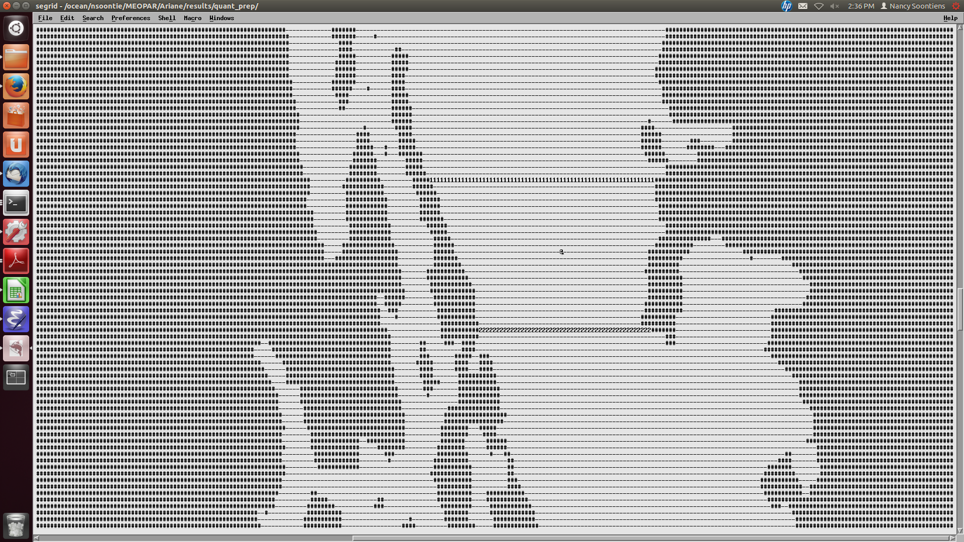
segrid: After you run mkseg0, you should see a new file calledsegrid. Edit this file with
nedit segrid
If you turn off text wrapping, you might see something like this:
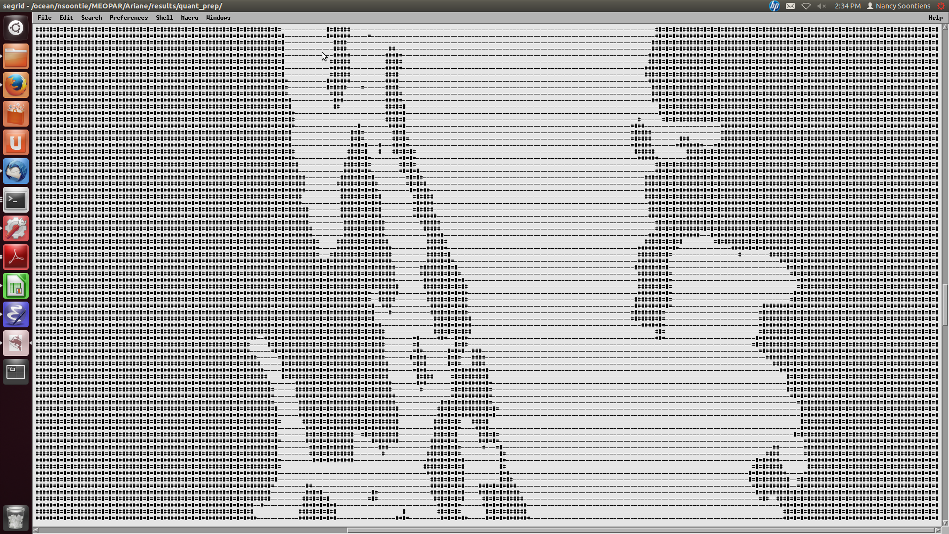
Land points are # and ocean points are -.
Add numbered sections to this file. Be sure your sections are over ocean points and not land points. Ariane will initialize particles along the section labelled as 1 and will calculate transport through all other sections. Your sections must make up a closed volume. Place the @ symbol somewhere within your closed subdomain. Your final edit might look something like this.
Run mkseg
mkseg
Copy the section definitions into a file called
sections.txt. The section definitions can be found from the output of mkseg.sections.txtshould look something like this:1 250 313 -409 -409 1 40 "1section" 2 264 312 386 386 1 40 "2section" 3 1 398 1 898 0 0 "Surface"
You can rename "1section" and "2section" to something more intuitive if you desire. You should also add a "Surface" section as above.
Run
ariane. Remember to check that you have added thearianeexecutable to your path.
ariane
The output on the screen should indicate that ariane completed successfully. You should also see a new file called
stats.txt. This file contains statistics about the initial and final particles through each section and the transport calculations. It might look something like this:total transport (in m3/s): 230033.88767527405 ( x lmt = 5520813.3042065771 ) max_transport (in m3/s) : 1000000000.0000000 # particles : 20380 initial state # 20380 stats. for: x y z a min: -123.457 48.946 0.500 0.000 max: -123.134 49.063 226.275 0.000 mean: -123.347 48.986 74.893 0.000 std. dev.: 0.062 0.022 61.722 0.000 meanders 166079.1572 0 1section .0000 1 2section 63952.7799 2 Surface .0000 3 total 230033.8877 except mnds 63954.7305 lost 1.9506 final state meanders # 11094 stats. ini: x y z a min: -123.457 48.946 0.500 0.006 max: -123.134 49.063 226.275 16.858 mean: -123.343 48.987 91.665 0.606 std. dev.: 0.055 0.020 61.438 1.010 stats. fin: x y z a min: -123.458 48.945 0.019 0.006 max: -123.132 49.064 238.621 16.858 mean: -123.329 48.992 91.483 0.606 std. dev.: 0.052 0.019 62.670 1.010 final state 2section # 9285 stats. ini: x y z a min: -123.457 48.946 0.500 0.191 max: -123.134 49.063 226.275 16.074 mean: -123.357 48.982 31.337 1.715 std. dev.: 0.075 0.028 35.675 1.639 stats. fin: x y z a min: -123.317 48.883 0.058 0.191 max: -123.079 48.970 151.722 16.074 mean: -123.192 48.929 25.504 1.715 std. dev.: 0.068 0.025 25.477 1.639
lost are the particles not intercepted by any section.
meanders are the particles that go back out the source section.
Time considerations
Particles initialized later in the simulation do not have as much time to cross one of the sections so it could be beneficial to impose a maximum age of each particle. This can be achieved by modifying mod_criter1.f90 in src/ariane as follows:
!----------------------------------------!
!- ADD AT THE END OF EACH LINE "!!ctr1" -!
!----------------------------------------!
!criter1=.FALSE.                 !! ctr1
!
!------------!
!- Examples -!
!------------!
!
     criter1=(abs(hl-fl).ge. lmt-lmax)   !! ctr1
lmt and lmax should be substituted by the values you set in the namelist.
You must remake and install ariane when making a change to any of the fortran files.
In
stats.txt, you will now see the particles intercepted by this time criterion.
meanders        135298.2260 0
1section        .0000 1
2section        13650.4035 2
Surface         .0000 3
Criter1         81085.2582 4
          total 230033.8877
    except mnds 94735.6616
           lost -.0000
Defining and tracking water masses
You can also impose a density and/or salinity and/or temperature criteria on the initial particles in order to track different water masses. You can achieve this by editing mod_criter0.f90.
!criter0=.TRUE.        !!ctr0
!
!------------!
!- Examples -!
!------------!
     criter0=(zinter(ss,hi,hj,hk,hl).le.29_rprec)     !!crt0
Once again, you must remake and install ariane.
You’ll also need to make sure that key_alltracers and key_computesigma are .TRUE. and zsigma are defined in your namelist.
Now particles will be initialized with salinity less than 29.
There are other examples of useful criteria in
mod_criter0.f90.Once again, the output of
stats.txtwill be different. Here is an example of part ofstats.txt:total transport (in m3/s): 76419.982459495324 ( x lmt = 1834079.5790278877 ) max_transport (in m3/s) : 1000000000.0000000 # particles : 16133 initial state # 16133 stats. for: x y z a t s r min: -123.457 48.946 0.500 0.000 4.693 16.243 13.336 max: -123.134 49.063 45.041 0.000 9.960 29.000 22.816 mean: -123.333 48.991 15.077 0.000 8.526 27.842 22.038 std. dev.: 0.075 0.027 10.570 0.000 0.973 1.458 1.040 meanders 26404.6357 0 1section 1057.5257 1 2section 12998.1853 2 Surface .0000 3 Criter1 35959.6357 4 total 76419.9825 except mnds 50015.3468 lost .0000
From the initial state statistics, you can see that the particles satisfy the salinity criteria. This might not be true of the final particles.
0ther files
Ariane will also produce netCDF files ariane_positions_quantitative.nc and ariane_statistics_quantitative.nc that can be used to plot the particle trajectories and statistics.