AMM12 Configuration Boundary Definition Analysis
22-Oct-2013 Susan Allen and Doug Latornell Salish Sea MEOPAR Project EOAS-UBC
This is an investigation of the differences in results obtained from runs of the AMM12 configuration with the unstructured boundaries (BDY) set via the 2 available mechanisms in NEMO-3.4:
using a
coordinates.bdy.ncfile (stock configuration)using a
nambdy_indexnamelist
The runs were done on salish using a 4x4 cores decomposition with no land processors specified.
Initial analysis found larger than expected differences in the temperature, u, and v values, and what looked like boundary effects in the difference plots on the south and west boundaries. Susan postulated that the difference was due to the order in which the boundaries are calculated in bdyini.F90 in contrast to the boundary order in the tide forcing files. Another run was done with a modified bdyini.F90. The results from that run are modbdy.
[1]:
%matplotlib inline
import netCDF4 as nc
import matplotlib.pyplot as plt
T-grid data:
[121]:
stock = nc.Dataset('stock/AMM12_30mn_20070101_20070101_grid_T.nc', 'r')
namlst = nc.Dataset('nambdy_index/AMM12_30mn_20070101_20070101_grid_T.nc', 'r')
modbdy = nc.Dataset('mod_bdyini/AMM12_30mn_20070101_20070101_grid_T.nc', 'r')
[123]:
for dim in stock.dimensions.itervalues(): print dim
<type 'netCDF4.Dimension'>: name = 'x', size = 198

<type 'netCDF4.Dimension'>: name = 'y', size = 224

<type 'netCDF4.Dimension'>: name = 'deptht', size = 33

<type 'netCDF4.Dimension'> (unlimited): name = 'time_counter', size = 48
Dimension of the nambdy_index results are the same, with the odd exception of the time_counter dimension which has size=47.
Some handy contour plotting functions:
[144]:
def conplot(data, t, d, var='votemper'):
    """Contour plot of var from data-set at time-step d
    and depth-step d.
    """
    field = data.variables[var]
    plt.contourf(field[t, d])
    plt.colorbar()

def diffplot(ref, other, t, d, var='votemper'):
    """Contour plot of difference ref[var] - other[var]
    at time-step t and depth-step d.
    """
    diff = ref.variables[var][t, d] - other.variables[var][t, d]
    plt.contourf(diff)
    plt.colorbar()
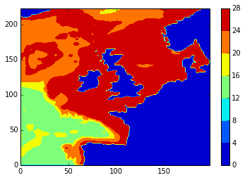
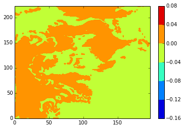
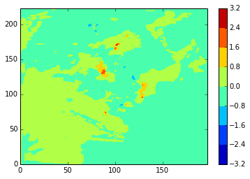
Just to get a feel for the results, here is the temperature field at the 5th depth level (note that depth uses s-coordinates) and the 46th time-step.
[145]:
conplot(namlst, 46, 5, var='votemper')
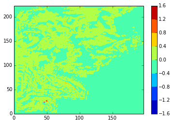
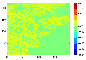
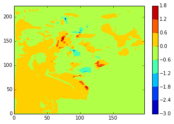
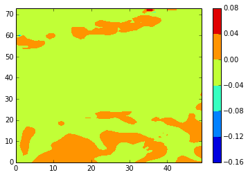
What we’re really interested in, though, is the differences. Here are diffs plots of temperature at the 24th time-step and 5th depth level. stock and modbdy show the least difference.
[146]:
diffplot(stock, namlst, 24, 5, var='votemper')
[147]:
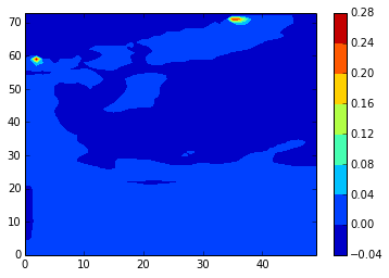
diffplot(stock, modbdy, 24, 5, var='votemper')
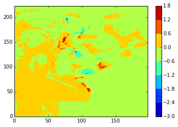
[148]:
diffplot(modbdy, namlst, 24, 5, var='votemper')

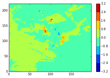
Now look at the differences in the velocity fields on the U and V grids.
[128]:
stock_u = nc.Dataset('stock/AMM12_30mn_20070101_20070101_grid_U.nc', 'r')
stock_v = nc.Dataset('stock/AMM12_30mn_20070101_20070101_grid_V.nc', 'r')
namlist_u = nc.Dataset('nambdy_index/AMM12_30mn_20070101_20070101_grid_U.nc', 'r')
namlist_v = nc.Dataset('nambdy_index/AMM12_30mn_20070101_20070101_grid_V.nc', 'r')
modbdy_u = nc.Dataset('mod_bdyini//AMM12_30mn_20070101_20070101_grid_U.nc', 'r')
modbdy_v = nc.Dataset('mod_bdyini/AMM12_30mn_20070101_20070101_grid_V.nc', 'r')
[129]:
diffplot(stock_u, namlist_u, 46, 5, var='vozocrtx')
[149]:
diffplot(stock_u, modbdy_u, 46, 5, var='vozocrtx')
[131]:
diffplot(modbdy_u, namlist_u, 46, 5, var='vozocrtx')
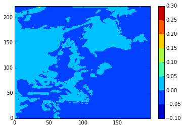
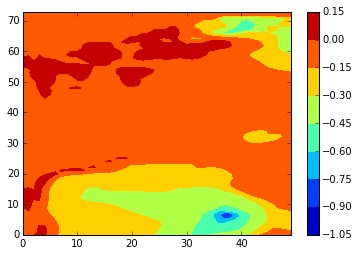
Again, stock and modbdy show the least difference, both in u (above) and v (below)
[115]:
diffplot(stock_v, namlist_v, 46, 5, var='vomecrty')
[150]:
diffplot(stock_v, modbdy_v, 46, 5, var='vomecrty')
[152]:
diffplot(modbdy_v, namlist_v, 46, 5, var='vomecrty')
Zooming the plots in to the upper left (near Iceland) corner:
[153]:
def z_conplot(data, t, d, var='votemper'):
    """Contour plot of var from data-set at time-step d
    and depth-step d.
    """
    field = data.variables[var]
    plt.contourf(field[t, d, 150:, :50])
    plt.colorbar()

def z_diffplot(ref, other, t, d, var='votemper'):
    """Contour plot of difference ref[var] - other[var]
    at time-step t and depth-step d.
    """
    diff = ref.variables[var][t, d] - other.variables[var][t, d]
    plt.contourf(diff[150:, :50])
    plt.colorbar()
[158]:
z_diffplot(stock_u, modbdy_u, 46, 5, var='vozocrtx')
[157]:
z_diffplot(stock_v, modbdy_v, 46, 5, var='vomecrty')
The v values (in contrast to the differences) appear to correspond to inconsistencies[1] noted in the AMM12 coordinates and tide forcing data files.
[1] nbit starts at 3, but the glamT value is for i=2
[154]:
z_conplot(modbdy_v, 46, 5, var='vomecrty')
[155]:
z_conplot(stock_v, 46, 5, var='vomecrty')

Our conclusion is that setting ln_coords_file to .false. in the namdby namelist so that the code in bdyini.F90 calculates the boundaries is a viable alternaive to constructing a coordinates.bdy.nc file for the Salish Sea case. Initially, the plan is to use:
nbdysege = 0
nbdysegw = -1
nbdysegn = -1
nbdysegs = 0
then evolve toward a partial boundary on the west and north sides of the domain.
Note that it is critical that the tide forcing boundary order be the same as that in bdyini.F90; i.e. east, west, north, south.